Introduction
A common misconception about randomized clinical trials is that the randomization process should balance any particular covariate across the arms of the trial and that therefore there is no benefit to controlling for covariates with a regression model unless a particular covariate happens to be unbalanced by chance. Determining whether a covariate is considered unbalanced amounts to performing a significance test comparing the arms and checking to see if the p-value is below some threshold (.05 for instance). This is wrong on two points.
Randomization does not ensure balance for any particular covariate. In fact it’s essentially certain that some covariates, measured or unmeasured, will be unbalanced. And secondly, even if the arms are “balanced” for a particular covariate ,in the sense of there being no significant difference across the arms, there is still value in adjusting for the covariate. Specifically, the more strongly related the covariate is with the outcome, the more beneficial the adjustment regardless of whether there is a significant difference. The nature of the benefit differs depending on whether the outcome being studied is continuous or binary and the measure being used.
Adjusting for predictive covariates of a continous outcome will result in the estimate being more precise. That is, smaller standard errors and confidence intervals. However, both the adjusted and unadjusted estimates are unbiased. This is not true of binary outcomes measures such as odds ratios (or for that matter hazard ratios). The unadjusted estimates are biased small, whereas the adjusted estimate has less bias but larger standard errors. The reduction in the bias (effect size increase) offsets the increase in standard errors so that there is an increase in power. This is an interesting phenomena worth exploring.
In this post I plan to perform some simple simulations demonstrating how estimates of a treatment effect can benefit from covariate adjustment of predictive yet “balanced” covariates for binary logistic regression models. This will also demonstrate the reduction in bias as well as increase in standard errors phenomena I mentioned above.
The setup
For the simulation I generated 1,000 pairs X1,X2 from a multivariate normal distribution with mean vector (0,0) and variance (10, 2), covariance (3). The variables are fairly correlated with \(\rho\) approximately .675. Next, I generated 1,000 bernoulli random variables with \(p = .5\). TRT = 1 represents whether the patient received the treatment variable and TRT = 0 means they received a placebo. The true data generating process is: \[logit(Y) = -2 + .15*X1 + 1.5*X2 - .5*TRT\]
Thus, we see that the true effect of the treatment is -.5 on the log odds scale, or a .61 odds ratio. Unadjusted and Adjusted estimates of TRT were obtained from the 1,000 randomly generated observations. This entire process was repeated 10,000 times so that each model was fit 10,000 times and 10,000 separate estimates were obtained for each model.
library(MASS)
library(ggplot2)
## Warning: package 'ggplot2' was built under R version 3.4.3set.seed(7521)
N <- 10000
Sigma <- matrix(c(10,3,3,2),2,2)
unadj.df <- data.frame(matrix(rep(NA, N*4), ncol = 4))
adj.df <- data.frame(matrix(rep(NA, N*4), ncol = 4))
unadj.OR <- adj.OR <- OR <- rep(NA, N)
for(i in 1:N){
X <- mvrnorm(1000, mu = c(0,0), Sigma = Sigma)
#simulate random assignment to a treatment
TRT <- rbinom(1000, size = 1, pr = .5)
#Probability of an event if everyone gets the treatment
trt.lo <- -2 + .15 * X[,1] + 1.5 * X[,2] - .5
trt.pr <- exp(trt.lo) / (1 + exp(trt.lo))
#Probability of an event if no one gets the treatment
pla.lo <- -2 + .15 * X[,1] + 1.5 * X[,2]
pla.pr <- exp(pla.lo) / (1 + exp(pla.lo))
#Generate binary outcomes
Y.trt <- rbinom(1000, size = 1, pr = trt.pr)
Y.pla <- rbinom(1000, size = 1, pr = pla.pr)
#Only observe actual assignment
Y <- ifelse(TRT == 1, Y.trt, Y.pla)
DAT <- data.frame(Y,TRT, X)
#True OR
OR[i] <- (mean(Y.trt)/(1 - mean(Y.trt))) /
(mean(Y.pla)/(1 - mean(Y.pla)))
#Fit models
unadj.mod <- glm(Y ~ TRT, family = binomial(link = "logit"), data = DAT)
unadj.df[i,] <- summary(unadj.mod)$coefficients[2,]
adj.mod <- glm(Y ~ X1 + X2 + TRT, family = binomial(link = "logit"), data = DAT)
adj.df[i,] <- summary(adj.mod)$coefficients[4,]
#Predict outcome with unadjusted model
newdata2 <- newdata <- DAT
newdata$TRT <- 1
newdata2$TRT <- 0
unadj.pr.trt <- predict(unadj.mod, newdata = newdata, type = "response")
unadj.pr.pla <- predict(unadj.mod, newdata = newdata2, type = "response")
unadj.OR[i] <- (mean(unadj.pr.trt) / (1 - mean(unadj.pr.trt))) /
(mean(unadj.pr.pla) / (1 - mean(unadj.pr.pla)))
adj.pr.trt <- predict(adj.mod, newdata = newdata, type = "response")
adj.pr.pla <- predict(adj.mod, newdata = newdata2, type = "response")
adj.OR[i] <- (mean(adj.pr.trt) / (1 - mean(adj.pr.trt))) /
(mean(adj.pr.pla) / (1 - mean(adj.pr.pla)))
}
names(unadj.df) <- c("Estimate", "SE", "Z", "P")
names(adj.df) <- c("Estimate", "SE", "Z", "P")
estimates <- data.frame(order = c(c(1:N),c(1:N)),
estimate = c(unadj.df[,1],adj.df[,1]),
SE = c(unadj.df[,2], adj.df[,2]),
P = c(unadj.df[,4], adj.df[,4]),
model = c(rep("unadjusted", N),rep("adjusted", N)))
#Color code if interval contains true value
estimates$contains <- with(estimates,
ifelse((estimate - 2*SE) > -.5 | (estimate + 2*SE) < -.5,
"No","Yes"))
#OR difference
ORD <- data.frame(ORD=c(OR - adj.OR, unadj.ORD = OR - unadj.OR),
model = c(rep("Adj",N),rep("Unadj",N)))Results
The results of the simulation are in line with what was stated above. The unadjusted estimate is biased low, has smaller standard errors, but also less power than the adjusted estimates. The proportion of adjusted confidence intervals (point estimate plus or minus 2 times the standard error) that contained the true treatment value of -.5 was a little over 95%. Whereas only 70% of the unadjusted confidence intervals contained the true value. About 69% of the the p-values for the adjusted estimate were below .05, but only 46% were for the unadjusted estimate.
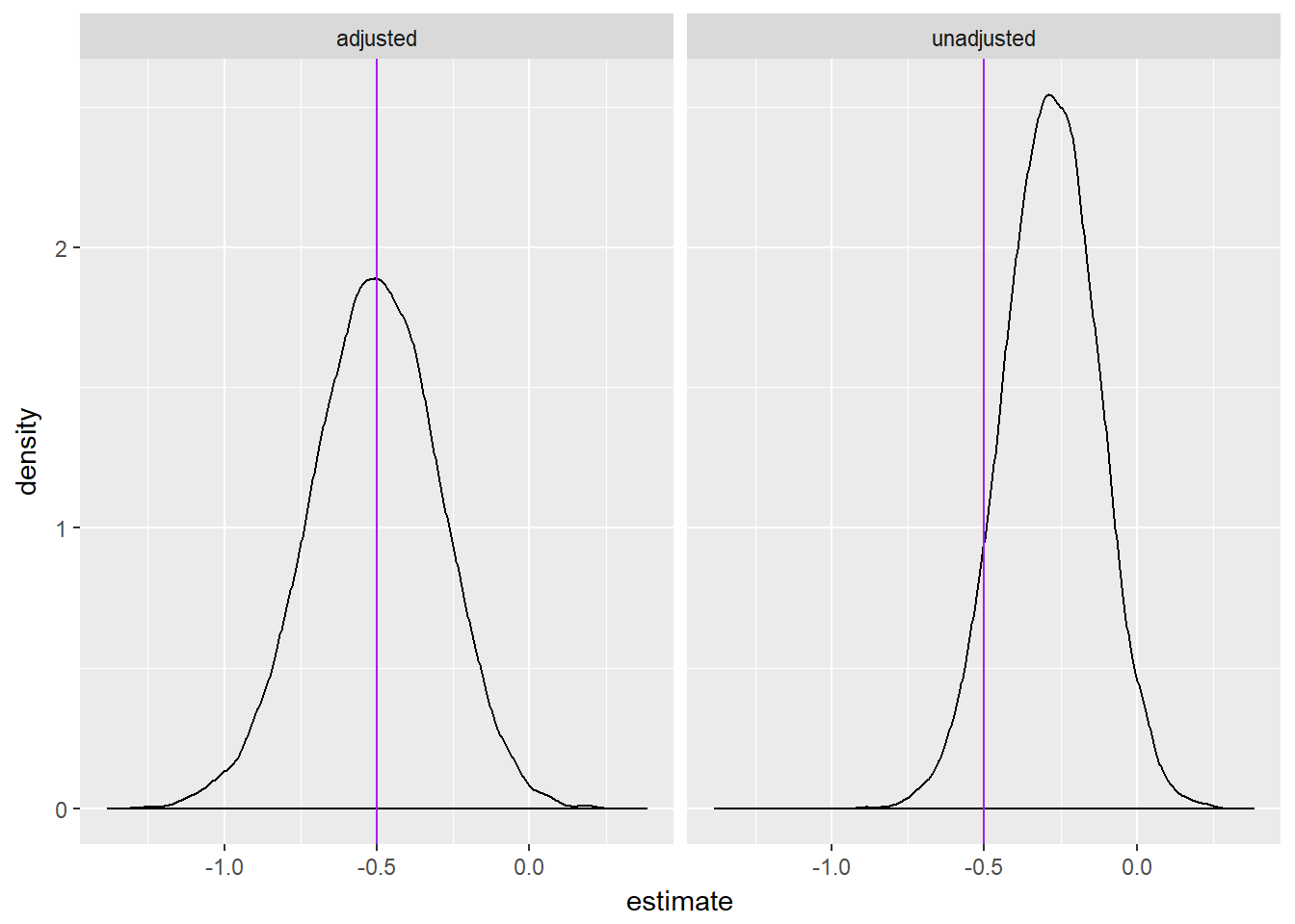
We can also inspect the the distribution of effect estimates for each model. The plots below show the distribution of effect estimates for all 10,000 simulations. Notice that the adjusted estimate is centered at the true value, whereas the unadjusted estimate is centered to the right (an underestimate).
ggplot(estimates, aes(estimate)) +
  geom_density() +
  geom_vline(xintercept = -.5, color = "purple") +
  facet_wrap(~ model)
The plot below displays the first 1000 simulations for each model. The black lines are the point estimate plus or minus two times the standard error. The lines that are red represent intervals that do not contain the true value, while black represents intervals that do contain the true value. Notice that almost all of the red lines for the unadjusted model are to the right, indicating that the estimate is too small.
ggplot(estimates[c(1:1000,10001:11000),], aes(x = estimate, y = order, color = contains)) +
  geom_point() +
  geom_errorbarh(aes(xmin=estimate - 2*SE, xmax= estimate + 2*SE), height=0.2, size=.5) +
  geom_vline(xintercept = -.5, color = "purple") +
  facet_wrap(  ~ model) +
  scale_color_manual(values=c("red","black")) +
  theme(axis.title.y=element_blank(),
        axis.text.y=element_blank(),
        axis.ticks.y=element_blank())
So it seems that, at least for this simple data set up, the adjusted model is clearly superior. I don’t know how these results hold up when the covariate adjusted model is mispecified, or when dealing with more complicated settings. These are topics I’d like to dig into in the future.
Additional Comments
It was correctly pointed out that since the odds ratio is non-collapsible (the conditional effect doesn’t necessarily equal the marginal effect), the unadjusted and adjusted estimates aren’t really estimating the same thing. The unadjusted estimate is estimating the marginal, or “population averaged” effect, while the adjusted model is estimating the conditional effect.
Thank you @analisereal - I was wondering if this was just the diff b/w marginal and conditional. @fledglingStat I love the simln, but why not add the counterfactual outcomes so you can get the marginal effect. e.g., for each observation create the y(trt=0) and y(trt=1)?
— Maria Glymour (@MariaGlymour) February 20, 2018
To explore what Dr. Glymour suggested, I added some code above that generates a separate “true” outcome for each patient, one under the treatment (Y.trt) and one under the control/placebo (Y.pla). Thus the true odds ratio is the ratio of the odds of these two values. The models are estimated using only the outcome value associated with the treatment assignment, since we only get to observe patients under one treatment regime (unless it’s a crossover design). Once the models were estimated I computed a predicted probability of an event both on an off the treatment for each patient and a corresponding odds ratio for each model. These serve as my marginal estimates. As is expected, the marginalized estimate for the unadjusted model is equal to coefficient in the unadusted regression model.
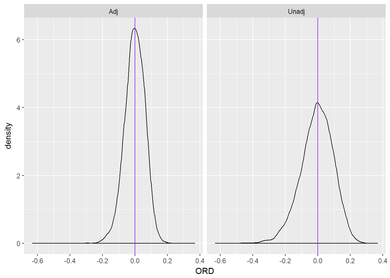
The plot below displays the distribution of differences between the true marginal odds ratio and the estimated marginal odds ratio for both models as well as a purple line at 0, representing no difference. I’ve also printed the mean difference for the unadjusted model followed by the adjusted model. From inspecting the plot it’s clear that both estimates are essentially unbiased, but the adjusted estimate is more steeply peaked with smaller tails. Thus, the adjusted estimate is less likely than the unadjusted estimate to produce a poor estimate, e.g. it generally lies closer to the truth.
ggplot(ORD, aes(ORD)) +
  geom_density() +
  geom_vline(xintercept = 0, color = "purple") +
  facet_wrap(~ model)
round(with(ORD,mean(ORD[model == "Unadj"])),3)## [1] -0.006round(with(ORD,mean(ORD[model == "Adj"])),3)## [1] -0.001