Contingency Tables and Simpson’s Paradox

Contingency tables are a way of representing the relationship between two or more categorical variables. Below is a 2x2 contingency with data from the indictments of 674 defendants involved in multiple murders in Florida from 1976 to 1987. The data is presented in Alan Agresti’s book “An introduction to categorical data analysis”. The table relates the death penalty verdict to the defendant’s race. The proportion of black defendants who received a “yes” verdict is p = 15/(176+15), or about 8%. The number of white defendants who received a “yes” verdict is p = 53/(430+53), or about 11%. This gives an odds ratio of (53x176)/(430x5) or about 1.45. This would appear to indicate that the odds for receiving the death penalty are higher for white defendants. However, this is not the case.

##                death_penalty  No Yes
## defendant_race                      
## Black                        176  15
## White                        430  53

What we have thus far considered is called a marginal association. If we extend our contingency table out to include another categorical variable we can consider what are called conditional associations. For instance, the tables below show defendant’s race and death penalty broken out by the victim’s race. This is what is mean by conditional, the value for victim’s race is held fixed and the association between the other variables is considered. For indictments involving black victim’s, the proportion of black defendants who received the death penalty is p = 4/(139+4), or about 3%. The proportion involving white defendants is 0/16, 0%. The odds ratio is (0x139)/(16x4) = 0. This seems to be the opposite of the marginal association considered above, where it seemed that white defendants were more likely to receive the death penalty.

What about the association for victim’s who are white? The proportion of black defendants is 11/(37+11) (23%) and white defendants is 53/(414+53) (11%). The odds ratio is (53x37)/(414x11) = .43. This shows the same flipped relationship as above! How is it that when ignoring the victim’s race, we see an increased odds of white defendants receiving the death penalty but that this associates completely flips when we condition on the victim’s race? This is an example of a famous statistical paradox referred to as Simpson’s paradox. A lot has been written about this paradox and I’m not going to rehash it here. The key lesson for now is to recognize that marginal associations can be very different from conditional associations and can lead to misleading inferences.

## , , victim_race = Black
## 
##               death_penalty
## defendant_race  No Yes
##          Black 139   4
##          White  16   0
## 
## , , victim_race = White
## 
##               death_penalty
## defendant_race  No Yes
##          Black  37  11
##          White 414  53

Risk and Odds

To my mind the most natural scale on which to interpret results for decision making is on the risk or probability scale. Why then talk about things like odds ratios when we could just consider risk differences, risk ratios (relative risk), etc? Well even though probability is a more natural scale for interpretation, this does not imply that it is the proper scale for analysis. The odds ratio and the log odds ratio (log here, as in most statistical applications, means natural logarithm) are often a more proper scale for analysis. Briefly, in any population where the underlying risk varies and the effect can be treated as constant on the log odds scale, reporting on the probability scale (risk difference, or relative risk) will probably not be appropriate since the estimates will vary see here. Maybe I’ll write a separate post expanding this argument.

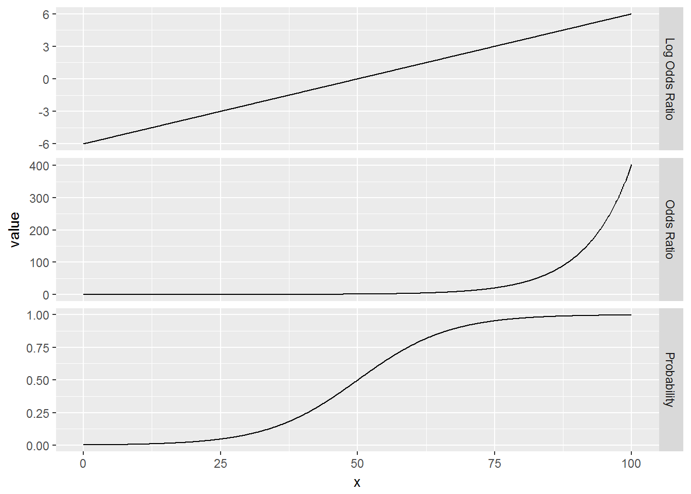
The dilemma then is that the scientifically relevant scale and the proper scale for analysis are not always the same. Thus, understanding each scale and how to translate back and forth is important. Below are three plots showing the relationship between an explanatory variable, ‘x’, and an outcome on the log odds scale, odds scale, and probability scale. The first thing that sticks out is that the plot of the log odds is a nice straight line. This shows that for a d unit change in x there is a constant change in the log odds. Notice also, that this is not true for the odds ratio or the probability scales. For instance, the probability at x = 20 is about .03, the probability at x = 30 is .08, and the probability at x = 40 is .23. The change in probability for a 10 unit change in x depends on where the change starts, i.e. the association is not “additive”" on these scales. This is also true of relative risk.

Logistic Regression

Logistic regression is an attractive way of extending regression techniques to binary data (though not the only way). Part of the attraction is the ease with which the model can be used to produce familiar measures like probability or odds ratios. conveniently, from a statistical perspective, the model is additive on the right scale (log odds). However, I’ve often noticed a fundamental misunderstanding as to which scale the model is additive on. Below is the implied relationship between covariates and outcome for logistic regressions on the probability scale, odds scale, and log odds scale.

#Marginal model for defendant suggests white victims more likely to get death penalty
mod1 <- glm(factor(death_penalty) ~  defendant_race,
              data = crime,
              family = binomial,
              weights = count)
summary(mod1)

## 
## Call:
## glm(formula = factor(death_penalty) ~ defendant_race, family = binomial, 
##     data = crime, weights = count)
## 
## Deviance Residuals: 
##      1       2       3       4       5       6       7       8  
## 15.305   7.481   0.000   4.511  -9.810  -2.460  -1.929  -4.768  
## 
## Coefficients:
##                     Estimate Std. Error z value Pr(>|z|)    
## (Intercept)          -2.4624     0.2690  -9.155   <2e-16 ***
## defendant_raceWhite   0.3689     0.3058   1.206    0.228    
## ---
## Signif. codes:  0 '***' 0.001 '**' 0.01 '*' 0.05 '.' 0.1 ' ' 1
## 
## (Dispersion parameter for binomial family taken to be 1)
## 
##     Null deviance: 440.84  on 6  degrees of freedom
## Residual deviance: 439.31  on 5  degrees of freedom
## AIC: 443.31
## 
## Number of Fisher Scoring iterations: 5

paste0("The odds ratio of white to black defendant's is ", round(exp(coef(mod1))[2],2))

## [1] "The odds ratio of white to black defendant's is 1.45"

#Probability of indictment if defendant is black
predict(mod1, newdata = data.frame(defendant_race = "Black"), type = "response")

##          1 
## 0.07853403

exp(-2.46)/(1 + exp(-2.46))

## [1] 0.07871034

#Probability of indictment if defendant is black
predict(mod1, newdata = data.frame(defendant_race = "White"), type = "response")

##         1 
## 0.1097308

exp(-2.4624 + .3689)/(1 + exp(-2.4624 + .3689))

## [1] 0.1097302

mod2 <- glm(factor(death_penalty) ~  defendant_race + victim_race,
              data = crime,
              family = binomial,
              weights = count)
summary(mod2)

## 
## Call:
## glm(formula = factor(death_penalty) ~ defendant_race + victim_race, 
##     family = binomial, data = crime, weights = count)
## 
## Deviance Residuals: 
##       1        2        3        4        5        6        7        8  
## 15.1995   5.6614   0.0000   5.3838  -9.9689  -4.4301  -0.6054  -2.7428  
## 
## Coefficients:
##                     Estimate Std. Error z value Pr(>|z|)    
## (Intercept)          -3.5961     0.5069  -7.095 1.30e-12 ***
## defendant_raceWhite  -0.8678     0.3671  -2.364   0.0181 *  
## victim_raceWhite      2.4044     0.6006   4.004 6.24e-05 ***
## ---
## Signif. codes:  0 '***' 0.001 '**' 0.01 '*' 0.05 '.' 0.1 ' ' 1
## 
## (Dispersion parameter for binomial family taken to be 1)
## 
##     Null deviance: 440.84  on 6  degrees of freedom
## Residual deviance: 418.96  on 4  degrees of freedom
## AIC: 424.96
## 
## Number of Fisher Scoring iterations: 5

paste0("The odds ratio of white to black defendant's is ", round(exp(coef(mod2))[2],2))

## [1] "The odds ratio of white to black defendant's is 0.42"

Logistic Regression: Interpreting multiple variables

Unlike standard linear regression models, interpreting logistic regressions with multiple variables can be tricky. This is directly related to the fact that it is only additive on the log odds scale, yet we typically want results presented on the odds or probability scales. Deriving the odds ratio is simple enough categorical variables, you just exponentiate the relevant coefficient from the model and this provides the odds ratio of that factor level relative to the reference category used in the model. For instance, in the model with defendant race and victim race the exponentiated coefficient for defendant race is .43. So the odds of receiving the death penalty are reduced by over half for white defendants relative to black defendants. Notice that this estimate is multiplicative, it essentially halves the odds of receiving the death penalty. It does not say anything about what the actual odds are. To estimate the odds, all the variables in the model need to be used. This can be seen by using some algebra on the odds ratio scale equation above.

\[ \frac{P(x)}{1 - P(x)} = exp(\beta_0 + \beta_1*x1 + \beta_2*x2) = exp(\beta_0)*exp(\beta_1*x1)*exp(\beta_2*x2)\]

What we see then is that estimating the odds requires a value specified for all of the variables in the model. It also provides an interpretation of the intercept on the odds scale, it’s the value of the odds when all the xs are set to 0 (because exp(0) = 1). In the case above, if we set the victim’s race to black then the odds are \(exp(-3.5961)*.42 = .027 * .42 = .011\). So the odds of receiving the death penalty when the victim is black and the defendant is black are about .027, which is then approximately halved to .011 if the defendant is white. Relatedly, when the victim is white and the defendant is black the odds are \(exp(-3.5961)*exp(2.4044) = .304\), these odds are again halved when the defendant is white, \(exp(-3.5961)*exp(2.4044)*.42 = .128\). Thus we see that the effects in a logistic regression are multiplicative on the odds scale.

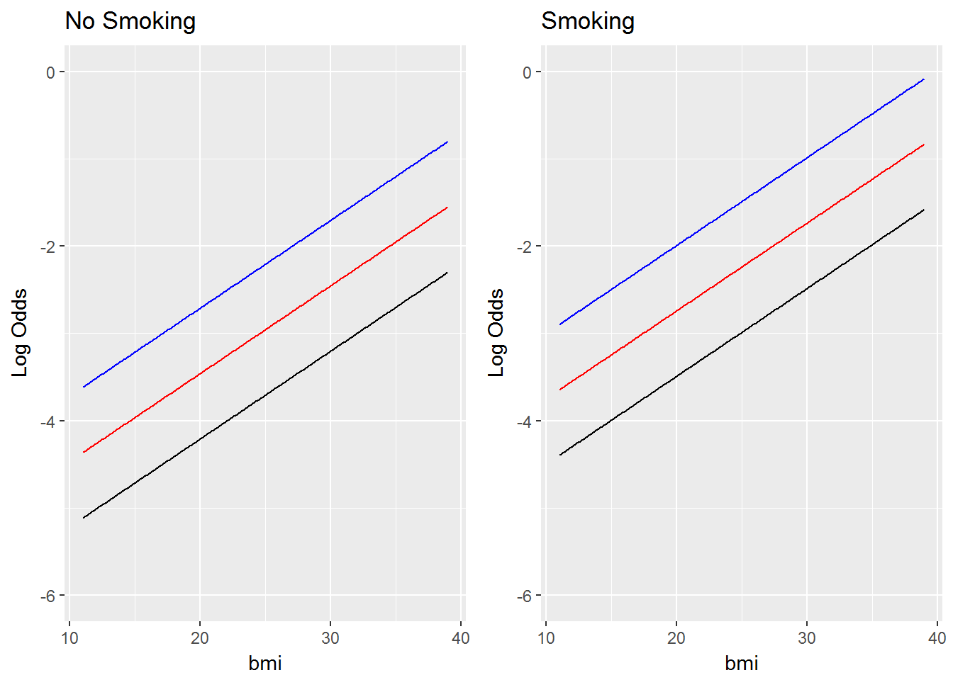
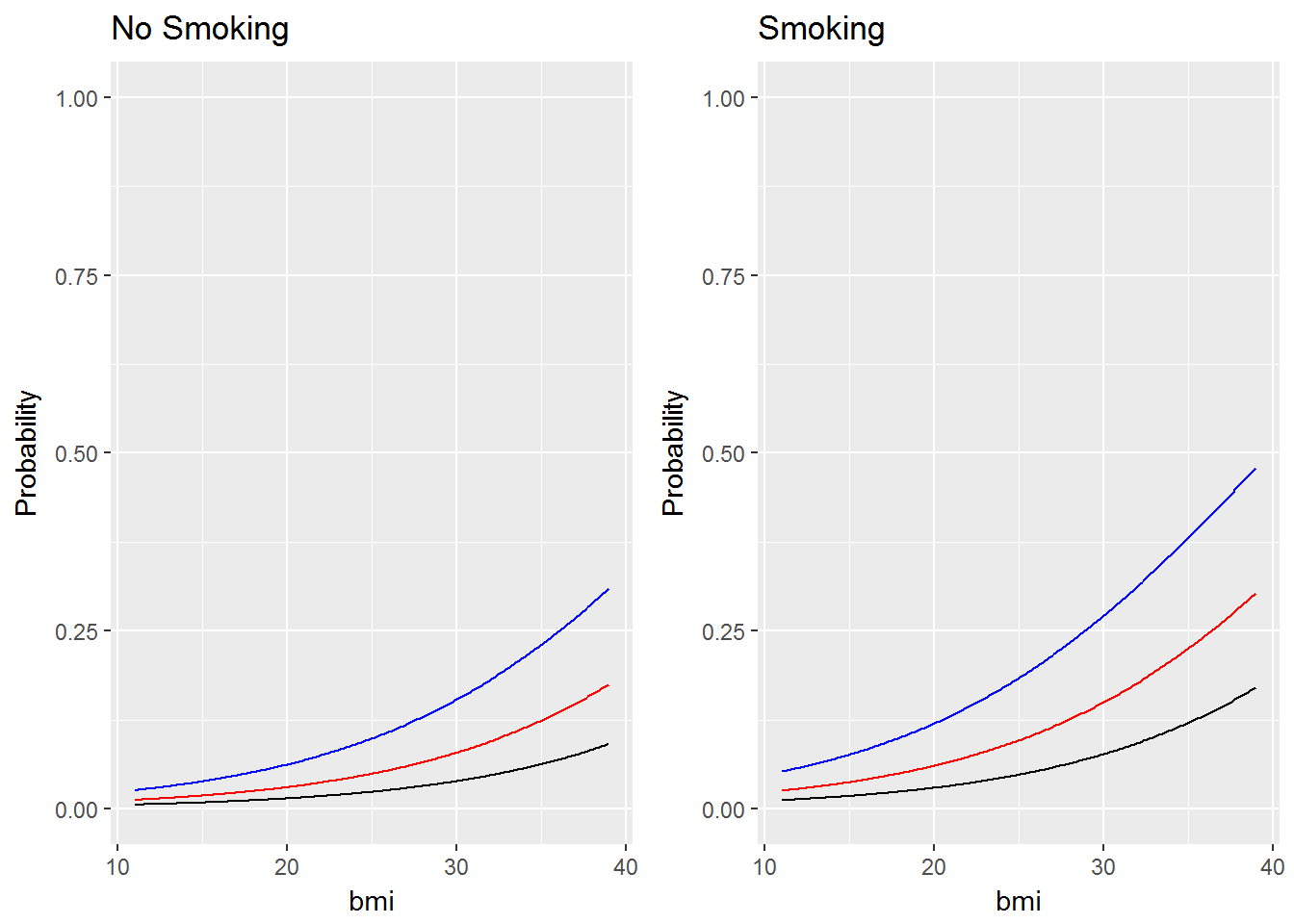
I fit a logistic regression model to the the WCGS dataset (Western Collaborative Group Study). The outcome is the occurrence of coronary heart disease. The explanatory variables I used are bmi, whether the subject smokes, and the subjects age. I’ve plotted the estimated log odds and probability as a function of bmi for at age = 35 (black lines), age = 45 (red lines), and age = 55 (blue lines) for both smokers and nonsmokers. What you will notice is that the log odds plot consists of straight lines, indicating constant additive effects as we expect from a regression model. However, on the probability scale it’s clear that the effects are not additive and that the effect of a 1 unit increase in bmi varies depending on whether the subject smokes and their age. The data is from the textbook “Regression Methods in Biostatistics” by Vittinghoff.

## 
## Call:
## glm(formula = factor(chd69) ~ 1 + bmi + smoke + age, family = binomial(), 
##     data = data)
## 
## Deviance Residuals: 
##     Min       1Q   Median       3Q      Max  
## -0.9670  -0.4487  -0.3656  -0.2867   2.7657  
## 
## Coefficients:
##             Estimate Std. Error z value Pr(>|z|)    
## (Intercept) -8.83969    0.84275 -10.489  < 2e-16 ***
## bmi          0.10047    0.02445   4.110 3.96e-05 ***
## smokeYes     0.71889    0.13669   5.259 1.45e-07 ***
## age          0.07491    0.01145   6.541 6.11e-11 ***
## ---
## Signif. codes:  0 '***' 0.001 '**' 0.01 '*' 0.05 '.' 0.1 ' ' 1
## 
## (Dispersion parameter for binomial family taken to be 1)
## 
##     Null deviance: 1781.2  on 3153  degrees of freedom
## Residual deviance: 1698.9  on 3150  degrees of freedom
## AIC: 1706.9
## 
## Number of Fisher Scoring iterations: 5