Yesterday I wrote a post using Stan to fit simple one parameter models. These are boring, but helpful for learning the basics. Today, I’d like to start building a series of increasingly complicated regression models. I have data on all the injuries that occured during the 2017 NFL (American Football) season, courtesy of https://www.armchairanalysis.com/. What I’d like to do is build a model to predict whether a player will have an injury, where I’m going to define injury as being listed at game time as out, or on injured reserve (IR) at any time during the season. I’m also going to restrict the analysis to a subset of positions: quarterbacks, running backs, tight ends, and wide receivers.
Creating the Analysis Data set
The code below creates a data set for every player who played (took at least 1 snap) in 2017 and information on whether the player was injured. Joining the tables was a bit tricky, so if you notice any issues please let me know. The four data sets I’m using (player, game, injury, offense) are from armchair analysis. I didn’t display the code loading them. The final data set has the player position and an indicator variable for whether they were injured (listed as out or IR at game time) anytime during the season.
#NFL Injury Data
library(tidyverse)
library(rstan)
options(tibble.print_max = 100)
#1. all players who were injured
#2. All players
#players who had any injury indication in 2017
inj.players <- game %>% filter(seas == 2017 & wk %in% c(1:17)) %>%
select(gid) %>% left_join(injury, by = c("gid" = "gid")) %>% select(player, gstat) %>%
mutate(injured = ifelse(gstat %in% c("IR", "Out"), 1, 0)) %>% group_by(player) %>%
summarize(games.inj = sum(injured)) %>% mutate(injured = ifelse(games.inj > 0, 1, 0)) %>%
left_join(player, by = c("player" = "player")) %>% select(player, pos1, games.inj, injured)
#All players who played an offensive snap in 2017
all.players <- game %>% filter(seas == 2017 & wk %in% c(1:17)) %>%
select(gid) %>% left_join(offense, by = c("gid" = "gid")) %>%
select(player) %>% left_join(player, by = c("player" = "player")) %>%
select(player, pos1) %>% group_by(player) %>% distinct()
#Join the two tables. Players who didn't get hurt will have missing values for injured
inj.data <- all.players %>% full_join(inj.players, by = c("player" = "player")) %>%
mutate(pos = ifelse(is.na(pos1.x),pos1.y,pos1.x)) %>%
ungroup() %>% select(pos,injured) %>%
filter(pos %in% c("QB","RB","TE","WR"))
#missing values for injured indicator should be 0
inj.data$injured[is.na(inj.data$injured)] <- 0
inj.data## # A tibble: 680 x 2
## pos injured
## <chr> <dbl>
## 1 RB 0
## 2 QB 0
## 3 TE 0
## 4 RB 1.00
## 5 RB 0
## 6 WR 0
## 7 WR 1.00
## 8 TE 1.00
## 9 RB 1.00
## 10 RB 0
## # ... with 670 more rowsFitting an intercept only model
Now that we have the data, I can fit a model. Normally I would do a little more exploratory analysis before moving to model fitting. The first model I’m going to fit is simply an intercept only logistic regression model. The prior on the intercept is a \(normal(0,5)\). The Stan code for this model is printed below. The generated quantities block generates values for posterior predictive checking. PPC involves comparing the posterior predictive distribution with the observed data, with the goal being to see whether there are issues with the model.
## data {
##   int<lower = 1> N;
##   int y[N];
## }
##
## //Intercept is the only parameter
## parameters {
##   real alpha;
## }
##
## model {
##   alpha ~ normal(0, 5);
##   y ~ bernoulli_logit(alpha);
## }
##
## generated quantities {
##   real p_hat_ppc = 0;
##
##   for (n in 1:N) {
##     int y_ppc = bernoulli_logit_rng( alpha);
##     p_hat_ppc = p_hat_ppc + y_ppc;
##   }
##   p_hat_ppc = p_hat_ppc / N;
## }
The function that fits the Stan model requires the data to be provided as a list.
#Fit intercept only model in Stan
#N is number of rows
data.list <- list(N = nrow(inj.data), y = inj.data$injured)

fit <- stan(file ='code\\intercept_LR.stan',
            data = data.list)
We can visually inspect the trace plot to check the sampling behavior of the markov chains used to construct the posterior. You want to see a nice mixing behavior, like those we get.
traceplot(fit)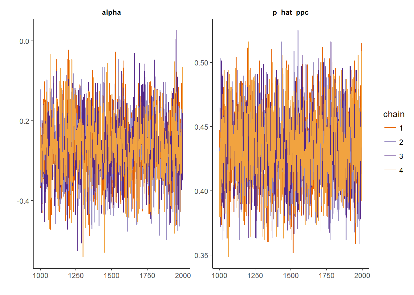
Before I move on to interpreting the model, I want to make sure that it fits well via posterior predictive checks. If I plot a histogram of predictived values of y (probability of injury) and over lay a vertical line corresponding to the overall proportion of injuries, it seems like the model has a great fit. However, we also have information about player position. In the second plot I overlay vertical lines for the proportion of injuries for all four positions in addition to the overall injury rate.
#Posterior Samples
params <- extract(fit)
#PPC
p_hat_ppc = data.frame(p_hat_ppc = params$p_hat_ppc)
OVERALL.mean <- mean(data.list$y)
QB.mean <- mean(data.list$y[inj.data$pos == "QB"])
RB.mean <- mean(data.list$y[inj.data$pos == "RB"])
TE.mean <- mean(data.list$y[inj.data$pos == "TE"])
WR.mean <- mean(data.list$y[inj.data$pos == "WR"])

ggplot(p_hat_ppc, aes(p_hat_ppc)) + geom_histogram(binwidth = 1/100) +
  geom_vline(aes(xintercept = OVERALL.mean, col = "black")) + theme_bw()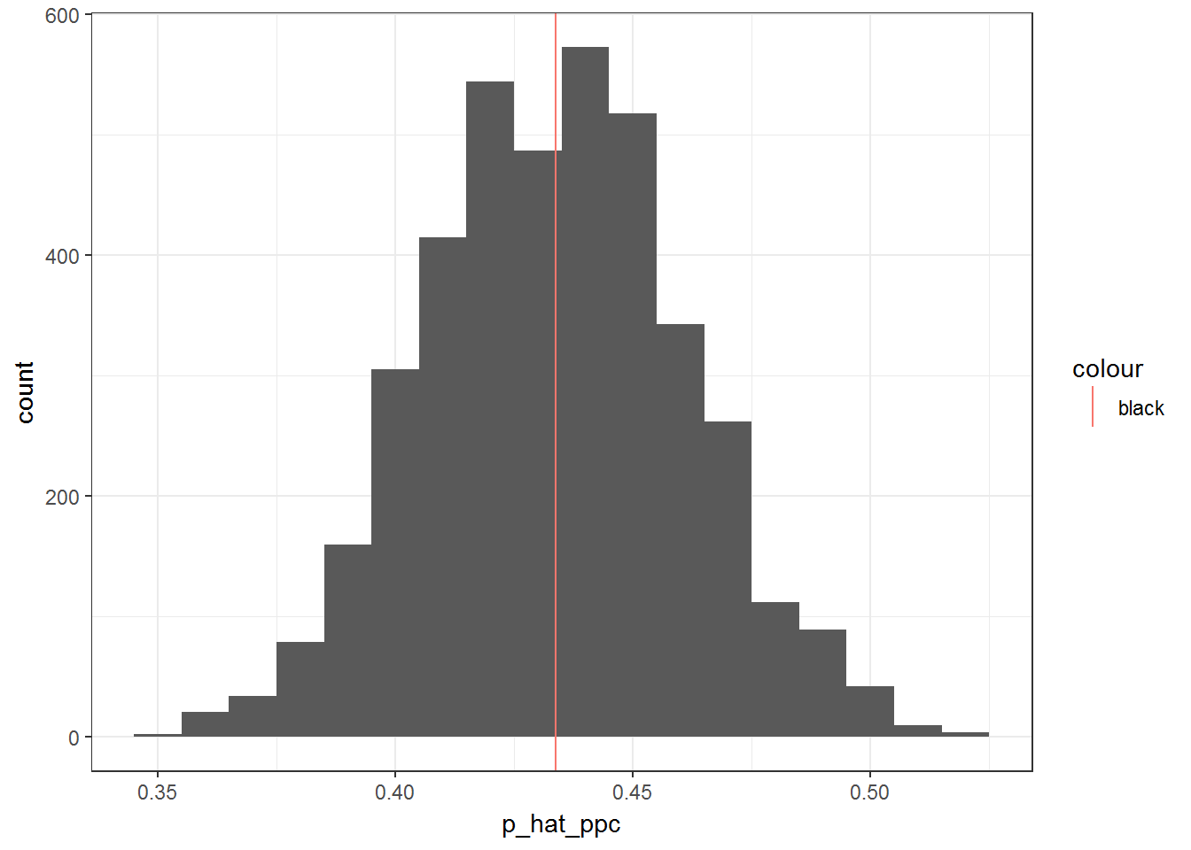
ggplot(p_hat_ppc, aes(p_hat_ppc)) + geom_histogram(binwidth = 1/100) +
  geom_vline(aes(xintercept = OVERALL.mean, col = "Overall")) +
  geom_vline(aes(xintercept = QB.mean, col = "QB")) +
  geom_vline(aes(xintercept = RB.mean, col = "RB")) +
  geom_vline(aes(xintercept = TE.mean, col = "TE")) +
  geom_vline(aes(xintercept = WR.mean, col = "WR")) +
  scale_color_manual(name = "Position",
                     values = c(Overall = "black",
                                QB = "red",
                                RB = "blue",
                                TE = "green",
                                WR = "purple")) +
  ggtitle("Posterior Predictive Distribution for Probability of Injury") +
  theme_bw()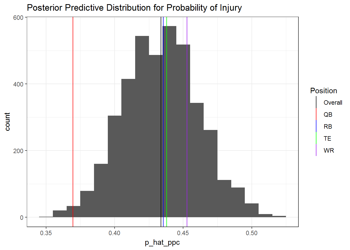
We can see from the second plot that the model would do very poorly for predicting quarterback injuries in particular. This suggests that a simple improvement to the model would be to include each players position.
Enriching the model with position information
Fitting a model in Stan with this information is fairly straight forward, but a little tricky. The key thing here is that our unknown parameters are a vector. I parameterized the model as a “cell means” model, so there is not intercept, just a mean parameter indexed by the four positions. You’ll notice that the generated quantities block is much longer now, since I had generate predictions for each position, as well as the overall.
## data {
##   int<lower = 1> N;
##   int<lower = 1> N_pos;
##   int<lower = 1, upper = 4> pos[N];
##   int y[N];
## }
##
## //alpha = intercept.
## parameters {
##   vector[N_pos] alpha;
## }
##
## model {
##   alpha ~ normal(0, 5);
##   y ~ bernoulli_logit(alpha[pos]);
## }
##
## generated quantities {
##   real p_hat_ppc = 0;
##   real p_hat_QB_ppc = 0;
##   real p_hat_RB_ppc = 0;
##   real p_hat_TE_ppc = 0;
##   real p_hat_WR_ppc = 0;
##
##   {
##     int n_QB = 0;
##     int n_RB = 0;
##     int n_TE = 0;
##     int n_WR = 0;
##
##     for (n in 1:N) {
##       int y_ppc = bernoulli_logit_rng(alpha[pos[n]]);
##
##       p_hat_ppc = p_hat_ppc + y_ppc;
##       if (pos[n] == 1) {
##         p_hat_QB_ppc = p_hat_QB_ppc + y_ppc;
##         n_QB = n_QB + 1;
##       }
##       else if (pos[n] == 2) {
##         p_hat_RB_ppc = p_hat_RB_ppc + y_ppc;
##         n_RB = n_RB + 1;
##       }
##       else if (pos[n] == 3) {
##         p_hat_TE_ppc = p_hat_TE_ppc + y_ppc;
##         n_TE = n_TE + 1;
##       }
##       else {
##         p_hat_WR_ppc = p_hat_WR_ppc + y_ppc;
##         n_WR = n_WR + 1;
##       }
##
##     }
##     p_hat_ppc = p_hat_ppc / (n_QB + n_RB + n_TE + n_WR);
##     p_hat_QB_ppc = p_hat_QB_ppc / n_QB;
##     p_hat_RB_ppc = p_hat_RB_ppc / n_RB;
##     p_hat_TE_ppc = p_hat_TE_ppc / n_TE;
##     p_hat_WR_ppc = p_hat_WR_ppc / n_WR;
##   }
## }
The model is fit the same as before except the data provided are a little different. N_pos is the number of levels to the positions variable (pos). Position is converted to a numeric vector where 1 = QB, 2 = RB, 3 = TE, 4 = WR. I’m not sure if Stan would automatically coerce the factor into numeric or not. Otherwise, N and y are the same. I use the same prior as before, \(normal(0,5)\), for the position effects.
#Fit model with position variable
data.list <- list(N = nrow(inj.data), N_pos = 4,
                  pos = as.numeric(factor(inj.data$pos)),
                  y = inj.data$injured)

fit2 <- stan(file ='code\\LR2.stan',
            data = data.list)
The traceplots as well as the posterior predictive checks for each position are below.
#Diagnostics
traceplot(fit2)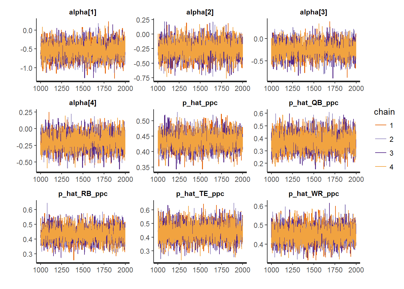
#Posterior Samples
params <- extract(fit2)

p_hat_ppc = data.frame(params)
head(p_hat_ppc)
## alpha.1 alpha.2 alpha.3 alpha.4 p_hat_ppc p_hat_QB_ppc
## 1 -0.4583329 -0.2061014 -0.455294597 -0.11832390 0.4338235 0.4021739
## 2 -0.7630776 -0.3645872 -0.233786211 -0.35338762 0.3676471 0.3152174
## 3 -0.4839392 -0.2106056 -0.069165609 -0.14304096 0.4573529 0.3478261
## 4 -0.7667736 0.1898111 -0.239908044 -0.27107444 0.4132353 0.3152174
## 5 -0.2340542 -0.1822146 0.004681824 0.08346487 0.5176471 0.4782609
## 6 -0.9798767 -0.2153992 -0.335015985 -0.26263767 0.4455882 0.3260870
## p_hat_RB_ppc p_hat_TE_ppc p_hat_WR_ppc lp__
## 1 0.4354839 0.3576642 0.4830189 -465.3913
## 2 0.4139785 0.3649635 0.3547170 -466.0841
## 3 0.4516129 0.5255474 0.4641509 -465.0915
## 4 0.4569892 0.4525547 0.3962264 -469.8522
## 5 0.5322581 0.4890511 0.5358491 -469.0604
## 6 0.4569892 0.4452555 0.4792453 -466.7845library(gridExtra)##
## Attaching package: 'gridExtra'## The following object is masked from 'package:dplyr':
##
## combineo <- ggplot(p_hat_ppc, aes(p_hat_ppc)) + geom_histogram(binwidth = 1/100) +
geom_vline(aes(xintercept = OVERALL.mean, col = "red")) + theme_bw()
a <- ggplot(p_hat_ppc, aes(p_hat_QB_ppc)) + geom_histogram(binwidth = 1/25) +
geom_vline(aes(xintercept = QB.mean, col = "red")) + theme_bw()
b <- ggplot(p_hat_ppc, aes(p_hat_RB_ppc)) + geom_histogram(binwidth = 1/25) +
geom_vline(aes(xintercept = RB.mean, col = "red")) + theme_bw()
c <- ggplot(p_hat_ppc, aes(p_hat_TE_ppc)) + geom_histogram(binwidth = 1/25) +
geom_vline(aes(xintercept = TE.mean, col = "red")) + theme_bw()
d <- ggplot(p_hat_ppc, aes(p_hat_WR_ppc)) + geom_histogram(binwidth = 1/25) +
geom_vline(aes(xintercept = WR.mean, col = "red")) + theme_bw()
grid.arrange(o,a,b,c,d)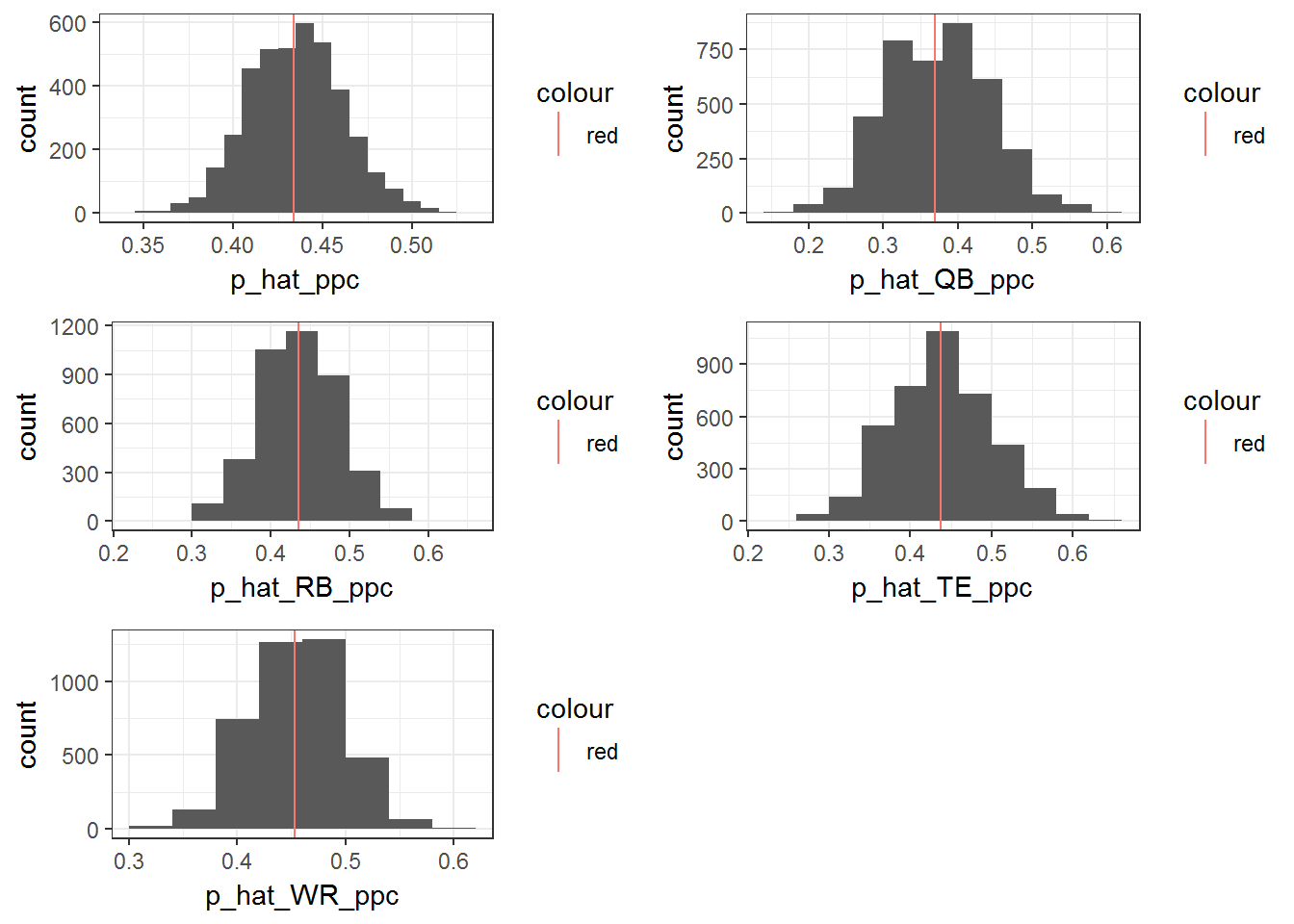
This model clearly improves the fit. Of course there must be more to the story than this. I hope to add more content to this post as I think more about the problem and the data I have available. For now, we can look at the marginal posterior distributions for each position.
a <- ggplot(p_hat_ppc, aes(exp(alpha.1))) + geom_histogram(binwidth = 1/100) +
  xlab("QB Effect") +
  theme_bw()
b <- ggplot(p_hat_ppc, aes(exp(alpha.2))) + geom_histogram(binwidth = 1/100) +
  xlab("RB Effect") +
  theme_bw()
c <- ggplot(p_hat_ppc, aes(exp(alpha.3))) + geom_histogram(binwidth = 1/100) +
  xlab("TE Effect") +
  theme_bw()
d <- ggplot(p_hat_ppc, aes(exp(alpha.4))) + geom_histogram(binwidth = 1/100) +
  xlab("WR Effect") +
  theme_bw()
grid.arrange(a,b,c,d)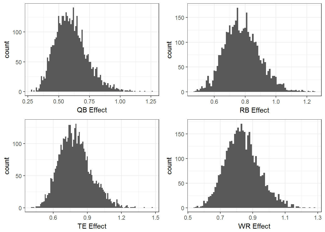
These last marginal plots show the estimated multiplicative effect of each position on even odds (probability 1/2 of an injury). The height of each histogram represents the relative plausibility of the effect. The majority of the mass for each position is below 1, suggesting that all these positions have a predicted injury rate less than .5.