Previously I use data from armchair analysis to build a simple model to predict whether an NFL player would have an injury based only on their position. I restricted the analysis to QBs, RBs, TEs, and WRs. In this post I’d like to expand the model to include 3 years of injury data (which is all I have), as well as include some additional covariates such as player height, weight, and age. The inclusion of multiple years of data makes building the model more tricky since some players will be included in each years’ data.
Additionally, I thought it would be more interesting to predict the number of games in a season a player is unable to play due to injury. A common model for counts is the poisson model. This model has a single parameter for its mean and variance, and so is not very flexible. It’s easy to imagine two simple processes by which a player can remain injury free all year. The first is they are simply lucky and don’t get hurt. The other is that they don’t play very much. Since there are (at least) two processes that can produce zeros for the number of games a player misses, I’m confident that there will be greater than expected number of zeros. Therefore it makes sense to include an additional parameter to account for this in the model.
To simplify the coding I’m going to use the excellent brms package in R. This package allows you to fit models in Stan using standard R formula syntax. It’ll also be helpful since it allows the use of splines to model potentially nonlinear predictors like height, weight, and age. Additionally, brms provides a ton of other functionality I’ll use. This post will be more involved than the previous one and so I’ve tried to split it into four sections: data pre-processing, exploratory analysis, statistical modeling, model comparison, and finally a simple simulation using the model.
Data Pre-Processing
The data for this analysis are different than the previous post primarily in two ways. The first is that it includes multiple years. This means that I will have more than one record (row) for players that played multiple years. The second is that I’m looking at the number of games missed due to injury. I’m defining an injury here as having a game time status of: out, physically unable to perform, or Injured Reserve. So essentially what I would like is a record for each year and each player with a number between 0 and 16 for games injured. The first 10 rows of the tables that need to be joined are printed below:
player## # A tibble: 10,139 x 27
## player fname lname pname pos1 pos2 height weight dob forty bench
## <chr> <chr> <chr> <chr> <chr> <chr> <int> <int> <chr> <dbl> <int>
## 1 AA-0025 Ameer Abdul~ A.Ab~ RB <NA> 69 205 6/13~ 4.50 24
## 2 AA-0050 Aaron Adams A.Ad~ OL <NA> 77 305 5/16~ 5.26 22
## 3 AA-0075 Andrew Adams A.Ad~ DB <NA> 71 203 10/2~ 4.54 24
## 4 AA-0100 Antho~ Adams A.Ad~ DL <NA> 72 300 6/18~ 5.13 0
## 5 AA-0200 Al Afala~ A.Af~ DB <NA> 71 212 1/20~ 4.48 25
## 6 AA-0300 Antho~ Alabi A.Al~ OL <NA> 77 315 2/16~ 5.12 18
## 7 AA-0400 Alex Albri~ A.Al~ LB <NA> 77 260 1/29~ 4.86 22
## 8 AA-0500 Allen Aldri~ A.Al~ LB <NA> 73 254 5/30~ 0 0
## 9 AA-0525 Alves~ Alexa~ A.Al~ RB <NA> 70 206 10/1~ 4.45 18
## 10 AA-0543 Adrian Amos A.Am~ DB <NA> 72 218 4/29~ 4.39 21
## # ... with 1.013e+04 more rows, and 16 more variables: vertical <dbl>,
## # broad <int>, shuttle <dbl>, cone <dbl>, arm <dbl>, hand <dbl>,
## # dpos <int>, col <chr>, dv <chr>, start <int>, cteam <chr>, posd <chr>,
## # jnum <int>, dcp <int>, nflid <int>, pimg <chr>game## # A tibble: 4,790 x 17
## gid seas wk day v h stad temp humd wspd wdir cond
## <int> <int> <int> <chr> <chr> <chr> <chr> <int> <int> <int> <chr> <chr>
## 1 1 2000 1 SUN SF ATL Geor~ 79 NA NA <NA> Dome
## 2 2 2000 1 SUN JAC CLE Clev~ 78 63 9 NE Sunny
## 3 3 2000 1 SUN PHI DAL Texa~ 109 19 5 S Sunny
## 4 4 2000 1 SUN NYJ GB Lamb~ 77 66 5 E Most~
## 5 5 2000 1 SUN IND KC Arro~ 90 50 8 E Most~
## 6 6 2000 1 SUN SEA MIA Pro ~ 89 59 13 E Sunny
## 7 7 2000 1 SUN CHI MIN Metr~ 65 NA NA <NA> Dome
## 8 8 2000 1 SUN TB NE Foxb~ 71 93 5 VAR Clou~
## 9 9 2000 1 SUN DET NO Loui~ 89 NA NA <NA> Dome
## 10 10 2000 1 SUN ARI NYG Gian~ 80 79 3 VAR Part~
## # ... with 4,780 more rows, and 5 more variables: surf <chr>, ou <dbl>,
## # sprv <dbl>, ptsv <int>, ptsh <int>injury## # A tibble: 15,862 x 6
## gid player team details pstat gstat
## <int> <chr> <chr> <chr> <chr> <chr>
## 1 3990 BS-4350 NE Concussion Did Not Participate In Practice Out
## 2 3990 TF-0750 NE Knee Full Participation in Practice Quest~
## 3 3990 TW-3250 NE Quadricep Limited Participation in Practice Quest~
## 4 3990 LJ-1250 PIT Concussion Did Not Participate In Practice Out
## 5 3991 JB-4550 CHI Ankle Limited Participation in Practice Quest~
## 6 3991 JB-8200 CHI Back Did Not Participate In Practice Proba~
## 7 3991 AJ-0430 CHI Calf Limited Participation in Practice Quest~
## 8 3991 EG-0350 CHI Concussion Full Participation in Practice Proba~
## 9 3991 JC-3100 CHI Concussion Full Participation in Practice Proba~
## 10 3991 MW-3250 CHI Hamstring Limited Participation in Practice Quest~
## # ... with 1.585e+04 more rowsoffense## # A tibble: 99,866 x 33
## uid gid player pa pc py ints tdp ra sra ry
## <int> <int> <chr> <int> <int> <int> <int> <int> <int> <int> <int>
## 1 1 1 KW-1500 0 0 0 0 0 0 0 0
## 2 2 1 CG-0400 0 0 0 0 0 15 7 62
## 3 3 1 JG-0600 36 23 252 1 3 2 1 22
## 4 4 1 JR-2000 0 0 0 0 0 1 0 - 2
## 5 5 1 TO-0200 0 0 0 0 0 0 0 0
## 6 6 1 FB-0200 0 0 0 0 0 5 2 10
## 7 7 1 JA-1600 0 0 0 0 0 24 10 77
## 8 8 1 CC-1400 31 16 264 0 2 4 1 12
## 9 9 1 BC-1100 0 0 0 0 0 3 0 5
## 10 10 1 TM-0900 0 0 0 0 0 0 0 0
## # ... with 9.986e+04 more rows, and 22 more variables: tdr <int>,
## # trg <int>, rec <int>, recy <int>, tdrec <int>, ret <int>, rety <int>,
## # tdret <int>, fuml <int>, peny <int>, conv <int>, fp <dbl>, fp2 <dbl>,
## # fp3 <dbl>, game <int>, seas <int>, year <int>, team <chr>, posd <chr>,
## # jnum <int>, dcp <int>, nflid <int>I join the tables using dplyr functions from the tidyverse package. In addition to the year, player, and number of games injured, I also get player name, weight, height, date of birth, as well as the year they entered the league (start).
#All games from 2015-2017
player.data <-
  data_frame(year = rep(2015:2017, each = 17),
                        wk = rep(1L:17L, times = 3)) %>%
  #Add game ids
  left_join(game %>% select(gid, seas, wk),
                        by = c("year" = "seas",
                               "wk" = "wk")) %>%
  #Add players with offense stats recorded in those years
  left_join(offense %>% select(gid,player), by = c("gid" = "gid")) %>%
  left_join(player %>% select(player,pname,pos1,height,weight,dob,start),
            by = c("player" = "player"))
#add injuries
injury.data <-
  data_frame(year = rep(2015:2017, each = 17),
             wk = rep(1L:17L, times = 3)) %>%
  #Add game ids
  left_join(game %>% select(gid, seas, wk),
            by = c("year" = "seas",
                   "wk" = "wk")) %>%
  left_join(injury %>% select(gid, player, gstat),
            by = c("gid" = "gid")) %>%
  left_join(player %>% select(player,pname,pos1,height,weight,dob,start),
            by = c("player" = "player")) %>%
  select(year,wk,gid,player,pos1,pname,height,weight,dob,start,gstat)
#Full data
full.data <-
  player.data %>% bind_rows(injury.data) %>%
  mutate(injured = ifelse(gstat %in% c("Out","IR","Pup","PUP", "Out\r"),1L,0L)) %>%
  select(year,player,pname,pos1,height,weight,dob,start,injured) %>%
  filter(pos1 %in% c("QB","RB","TE","WR")) %>%
  group_by(year,player,pname,pos1,height,weight,dob,start) %>%
  summarize(games.inj = sum(injured)) %>% unique()

#Age variable
full.data$age <- full.data$year - lubridate::year(as.Date(full.data$dob, "%m/%d/%Y"))
The table I’ll use for analysis is printed here.
full.data## # A tibble: 1,908 x 10
## # Groups: year, player, pname, pos1, height, weight, dob [1,908]
## year player pname pos1 height weight dob start games.inj age
## <int> <chr> <chr> <chr> <int> <int> <chr> <int> <int> <dbl>
## 1 2015 AA-0025 A.Abdul~ RB 69 205 6/13/~ 2015 0 22.0
## 2 2015 AA-1350 A.Andre~ RB 70 225 10/15~ 2014 1 23.0
## 3 2015 AB-1975 A.Blue RB 74 223 4/27/~ 2014 0 24.0
## 4 2015 AB-2000 A.Boldin WR 73 220 10/3/~ 2003 0 35.0
## 5 2015 AB-2600 A.Brads~ RB 69 214 3/19/~ 2007 0 29.0
## 6 2015 AB-3500 A.Brown WR 70 186 7/10/~ 2010 0 27.0
## 7 2015 AC-0100 A.Caldw~ WR 72 200 4/15/~ 2008 0 30.0
## 8 2015 AC-1650 A.Cleve~ TE 77 258 3/21/~ 2014 0 23.0
## 9 2015 AC-2350 A.Cooper WR 73 211 6/17/~ 2015 0 21.0
## 10 2015 AD-0100 A.Dalton QB 74 215 10/29~ 2011 3 28.0
## # ... with 1,898 more rowsBefore modeling the data, it’s always good to do some quality checks. Exploratory analysis can be very helpful in this regard since it can help identify irregularities and other issues with the data. Prior knowledge can be helpful here as well. For instance I know how many games some of my favorite players have missed in the last three seasons and I can use that as a standard to check the data against.
Le’veon Bell is one of my favorite players (I’m of course a Steelers fan) and I know that he hurt his knee is 2015 and missed most of the season. Let’s check the data set I created to make sure it contains this information. Bell’s player unique player id in this data set is “LB-0250”. We can select only the rows with his id by using the filter function from dplyr.
filter(full.data, player == "LB-0250")## # A tibble: 3 x 10
## # Groups: year, player, pname, pos1, height, weight, dob [3]
## year player pname pos1 height weight dob start games.inj age
## <int> <chr> <chr> <chr> <int> <int> <chr> <int> <int> <dbl>
## 1 2015 LB-0250 L.Bell RB 73 230 2/18/1992 2013 0 23.0
## 2 2016 LB-0250 L.Bell RB 73 230 2/18/1992 2013 0 24.0
## 3 2017 LB-0250 L.Bell RB 73 230 2/18/1992 2013 0 25.0Well that’s not good. The data set says Bell didn’t miss any games in 2015, even though we know he did. Before rechecking the code I used to join the tables, let’s look at the entries for Bell in the full injury data set. If it’s missing there then the data I have is simply incomplete.
filter(injury, player == "LB-0250")## # A tibble: 3 x 6
## gid player team details pstat gstat
## <int> <chr> <chr> <chr> <chr> <chr>
## 1 4271 LB-0250 PIT Suspension <NA> Suspend
## 2 4275 LB-0250 PIT Suspension <NA> Suspend
## 3 4301 LB-0250 PIT Suspension <NA> SuspendIt looks like the raw data simply doesn’t have the information recorded! There must be something going on then with how the injury data was recorded. There are other omissions in the raw injury data set that I discovered as well. It would be too time consuming to fix all of them, so I’m simply going to proceed with the analysis, however this means anything that follows is obviously suspect.
Exploratory Analysis
Simple summaries are an effective way of exploring your data and can help diagnose potential issues. A simple summary table of the data is printed below.
summary(full.data)## year player pname pos1 height
## Min. :2015 AA-0025: 3 Length:1908 QB:247 Min. :66.00
## 1st Qu.:2015 AB-1975: 3 Class :character RB:538 1st Qu.:71.00
## Median :2016 AB-3500: 3 Mode :character TE:400 Median :73.00
## Mean :2016 AC-1650: 3 WR:723 Mean :73.22
## 3rd Qu.:2017 AC-2350: 3 3rd Qu.:76.00
## Max. :2017 AD-0100: 3 Max. :80.00
## (Other):1890
## weight dob start games.inj
## Min. :149 Length:1908 Min. :1994 Min. : 0.000
## 1st Qu.:200 Class :character 1st Qu.:2011 1st Qu.: 0.000
## Median :217 Mode :character Median :2013 Median : 0.000
## Mean :219 Mean :2013 Mean : 1.327
## 3rd Qu.:236 3rd Qu.:2015 3rd Qu.: 1.000
## Max. :283 Max. :2017 Max. :16.000
##
## age
## Min. :17.00
## 1st Qu.:24.00
## Median :25.00
## Mean :26.19
## 3rd Qu.:28.00
## Max. :58.00
## NA's :3From examining the table, a few things immediately pop out. The max age is 58 years old! And someone has 1994 listed as the year they entered the league. I’ll spare you the boring details, but essentially several new players share names with previous players and some how their information has gotten mixed up. For instance this profile on NFL.com for WR George Farmer (the culprit in our data set) has his age listed as 59 years old. The player in our data set is also listed as a WR. I updated the data set to reflect what I think are the correct values, 24 year old running back. The ages are missing for 3 players as well. They all recently entered the league, so I simply assume they are 23 years old.
There is also a Charles Johnson, WR, who was born 1972. I’m pretty sure this is actually a player who was born in 1989 and now plays for the jets and not the Charles Johnson that won a superbowl with the Patriots in the early 2000s. Another WR name Trevor Davis also had an incorrect age. I manually corrected these records.
Simple plots should help to identify if there are any other data issues. I produce several plots below.
####Exploratory Analysis####
full.data %>% group_by(games.inj) %>%
  summarize(FREQ = n()) %>%
  ggplot(aes(x = games.inj, y = FREQ)) + geom_point()
full.data %>% group_by(games.inj, pos1) %>%
  summarize(FREQ = n()) %>%
  ggplot(aes(x = games.inj, y = FREQ, col = pos1)) + geom_point()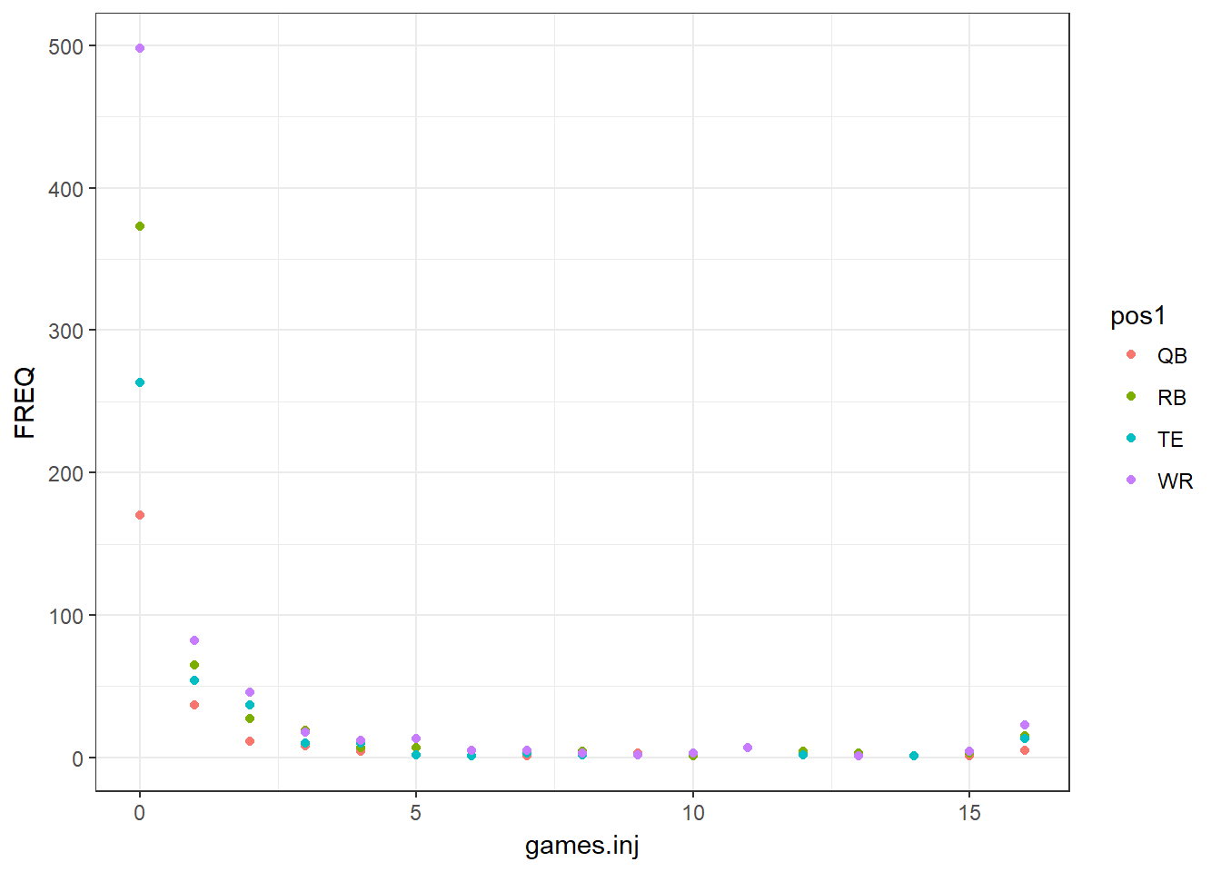
full.data %>% group_by(pos1) %>% mutate(total_pos = n()) %>%
  ungroup() %>% group_by(games.inj, pos1) %>%
  mutate(FREQ = n(),
         proportion = FREQ/total_pos) %>%
  ggplot(aes(x = games.inj, y = proportion, col = pos1)) + geom_line()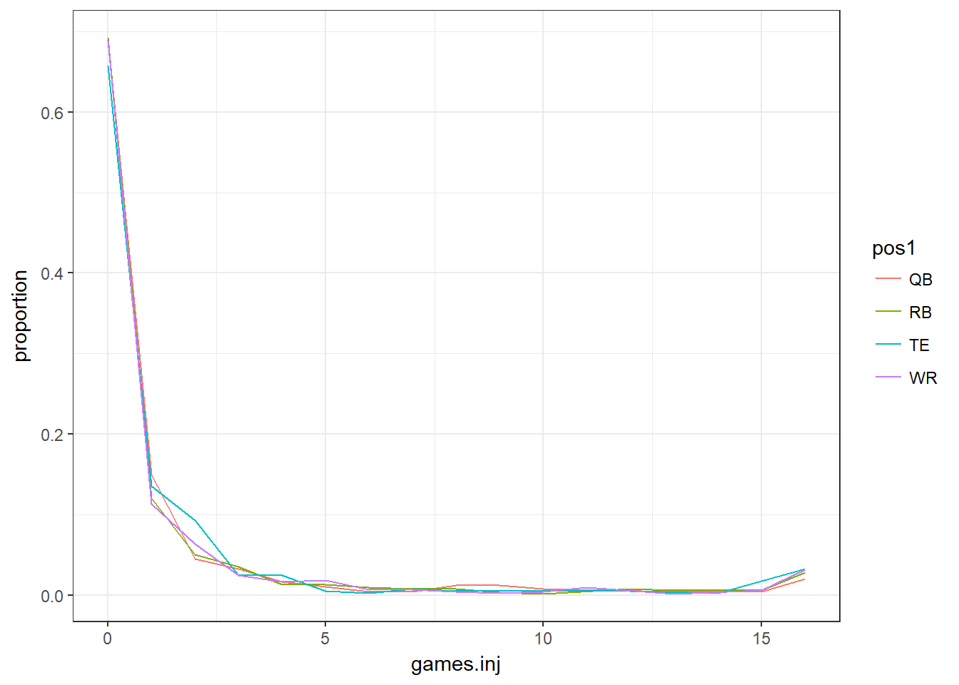
full.data %>% group_by(year,games.inj,pos1) %>%
  ggplot(aes(pos1, games.inj)) + geom_boxplot() + facet_wrap( ~ year)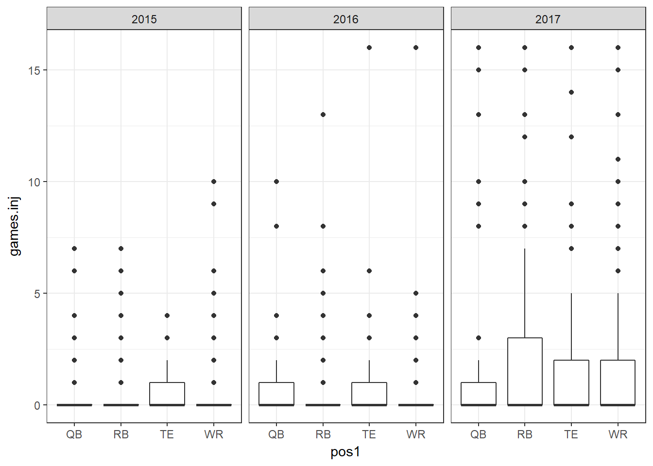
#Injuries by year
#Vast majority of injuries occur in 2017
full.data %>% group_by(year) %>% summarize(total = sum(games.inj)) %>%
  ggplot(aes(y = total, x = year)) + geom_point()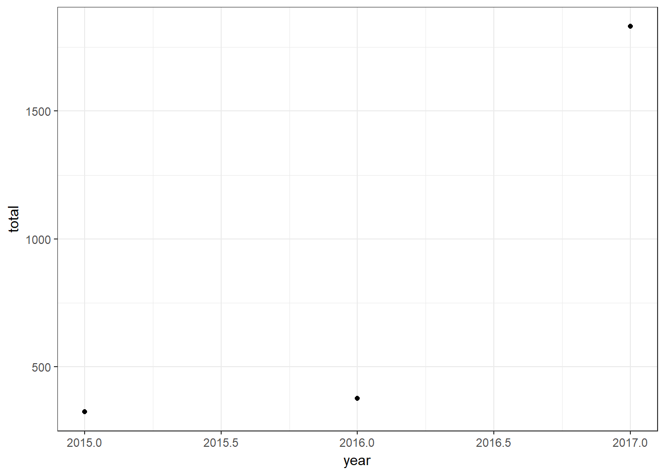
The last graph really sticks out to me. I see no reason for there to be a substantial differences in the number of injuries from 2015 to 2017. My guess is that the veracity of the data declines from 2017 backward. This coheres with the missing injury checks above. The years I found missing injuries were from either 2015 or 2016. I think this implies that I should only model the 2017 data. I’m going to ignore this sound advice simply because I want to get some practice fitting complex models with brms, but all the results should be taken with a grain of salt (or maybe an entire shaker).
Statistical Modeling
Zero Inflated Poisson
The first model I’m going to fit is a zero inflated poisson. This model is a mixture of two models. A binomial model that estimates the probability of missing zero games and a separate poisson model to estimate the number of games missed. Zeros can then be produced by both processes. The binomial model only uses year and position to estimate the probability of zero. The poisson model uses zero, position, player height, weight, and age. Additionally, the poisson model has a random intercept for each player to account for the correlation across years. Simple mathematical representations of the models are presented below. I stick an exponential prior with rate parameter = 2 to impose some regularization on the varying player intercepts. This factor has over 900 levels and at most 3 observations per level. \[Y \sim ZIPoisson(p_i, \lambda_i) \] \[logit(p_i) \sim \alpha_p + \beta_p*X \] \[log(\lambda_i) \sim \alpha_\lambda + \alpha_{player_p} + \beta_\lambda*X \] \[\alpha_{\lambda} \sim Normal(0,10)\] \[\alpha_z \sim Normal(0,1)\] \[\beta_\lambda, \beta_z \sim Normal(0,1) \] \[\alpha_{player_\lambda} \sim Normal(0,sd_\lambda)\] \[sd_\lambda \sim exponential(2)\]
fit0 <- brm(bf(games.inj ~ year + pos1 + height + weight + age + (1|player),
               zi ~ 1),
            data = full.data, family = zero_inflated_poisson(link = "log"),
            prior = c(set_prior("normal(0, 5)", class = "Intercept"),
                      set_prior("normal(0,.5)", class = "Intercept", dpar = "zi"),
                      set_prior("normal(0, 1)", class = "b"),
                      set_prior("exponential(2)", class = "sd")),
            cores = 4)
summary(fit0)
## Family: zero_inflated_poisson
## Links: mu = log; zi = logit
## Formula: games.inj ~ year + pos1 + height + weight + age + (1 | player)
## zi ~ 1
## Data: full.data (Number of observations: 1908)
## Samples: 4 chains, each with iter = 2000; warmup = 1000; thin = 1;
## total post-warmup samples = 4000
## ICs: LOO = NA; WAIC = NA; R2 = NA
##
## Group-Level Effects:
## ~player (Number of levels: 959)
## Estimate Est.Error l-95% CI u-95% CI Eff.Sample Rhat
## sd(Intercept) 1.18 0.07 1.04 1.32 648 1.00
##
## Population-Level Effects:
## Estimate Est.Error l-95% CI u-95% CI Eff.Sample Rhat
## Intercept -1440.29 105.04 -1650.41 -1232.46 1905 1.00
## zi_Intercept 0.05 0.09 -0.12 0.23 1186 1.00
## year 0.72 0.05 0.61 0.82 1898 1.00
## pos1RB 0.15 0.25 -0.34 0.64 696 1.00
## pos1TE 0.36 0.24 -0.13 0.82 740 1.00
## pos1WR 0.05 0.22 -0.37 0.48 753 1.00
## height -0.00 0.04 -0.09 0.08 526 1.01
## weight -0.01 0.01 -0.02 0.00 523 1.01
## age 0.01 0.02 -0.03 0.04 673 1.00
##
## Samples were drawn using sampling(NUTS). For each parameter, Eff.Sample
## is a crude measure of effective sample size, and Rhat is the potential
## scale reduction factor on split chains (at convergence, Rhat = 1).Posterior Predictive Checks
pp_check(fit0, nsamples = 20) + xlim(c(0,16))## Warning: Removed 373 rows containing non-finite values (stat_density).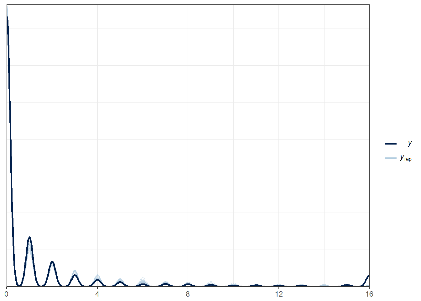
pp_check(fit0, nsamples = 20, type = "ecdf_overlay")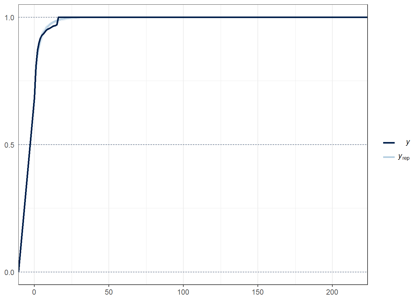
The zero inflated poisson model seems to fit the data fairly well except for those players who missed 16 games. It’s conceivable that there is a third process at work which determines whether a player will miss 16 games, namely that they suffer a season ending injury in the off-season or pre-season. Stan would allow us to create a mixture distribution like the zero inflated poisson.
For simplicity (i.e. I’m lazy) I’m instead going to divide the number of games missed by 16, which transforms the outcome into the proportion of games missed out of 16. This allows us to fit a zero-one inflated beta regression. This model is a mixture distribution like the zero inflated poisson, except there are now two binomial processes that account for the values 0 and 1. The beta distribution is then used as the model for all values in between. One big issue with this model is that it’s continuously valued between the (0,1) interval, where as our data were originally integers.
Zero-One Inflated Beta
#zero-one inflated beta
full.data$prop.inj <- full.data$games.inj/16

fit1 <- brm(bf(prop.inj ~ year + pos1 + height + weight + age + (1|player),
               coi ~ 1,
               zoi ~ 1),
            data = full.data, family = zero_one_inflated_beta(),
            prior = c(set_prior("normal(0, 5)", class = "Intercept"),
                      set_prior("normal(0,.5)", class = "Intercept", dpar = "zoi"),
                      set_prior("normal(0,.5)", class = "Intercept", dpar = "coi"),
                      set_prior("normal(0,1)", class = "b"),
                      set_prior("exponential(2)", class = "sd")),
            cores = 4)
summary(fit1)
## Family: zero_one_inflated_beta
## Links: mu = logit; phi = identity; zoi = logit; coi = logit
## Formula: prop.inj ~ year + pos1 + height + weight + age + (1 | player)
## coi ~ 1
## zoi ~ 1
## Data: full.data (Number of observations: 1908)
## Samples: 4 chains, each with iter = 2000; warmup = 1000; thin = 1;
## total post-warmup samples = 4000
## ICs: LOO = NA; WAIC = NA; R2 = NA
##
## Group-Level Effects:
## ~player (Number of levels: 959)
## Estimate Est.Error l-95% CI u-95% CI Eff.Sample Rhat
## sd(Intercept) 0.06 0.05 0.00 0.18 1983 1.00
##
## Population-Level Effects:
## Estimate Est.Error l-95% CI u-95% CI Eff.Sample Rhat
## Intercept -495.65 99.30 -696.45 -296.50 4000 1.00
## zoi_Intercept 0.90 0.05 0.80 1.00 4000 1.00
## coi_Intercept -2.96 0.12 -3.20 -2.73 4000 1.00
## year 0.24 0.05 0.15 0.34 4000 1.00
## pos1RB 0.16 0.17 -0.16 0.49 4000 1.00
## pos1TE 0.07 0.16 -0.25 0.37 4000 1.00
## pos1WR 0.06 0.14 -0.20 0.34 4000 1.00
## height 0.00 0.03 -0.05 0.05 4000 1.00
## weight -0.00 0.00 -0.01 0.00 4000 1.00
## age 0.02 0.01 0.00 0.05 4000 1.00
##
## Family Specific Parameters:
## Estimate Est.Error l-95% CI u-95% CI Eff.Sample Rhat
## phi 5.01 0.30 4.45 5.63 4000 1.00
##
## Samples were drawn using sampling(NUTS). For each parameter, Eff.Sample
## is a crude measure of effective sample size, and Rhat is the potential
## scale reduction factor on split chains (at convergence, Rhat = 1).I’m more familiar with the zero inflated poisson so I’m going to stick with the zero inflated poisson, even though it doesn’t account for the increased prevalence of missing 16 games.
Simple Interpretation
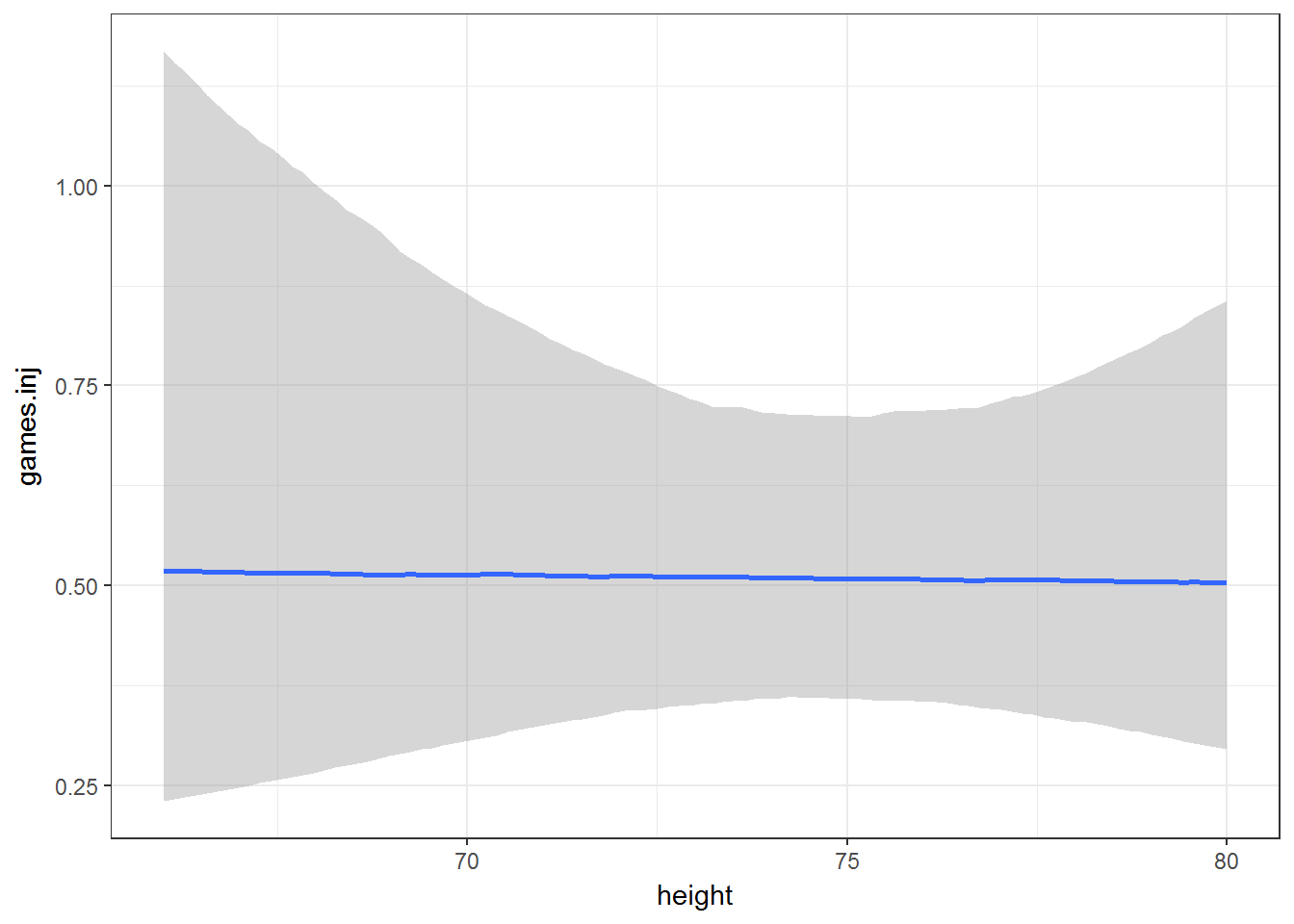
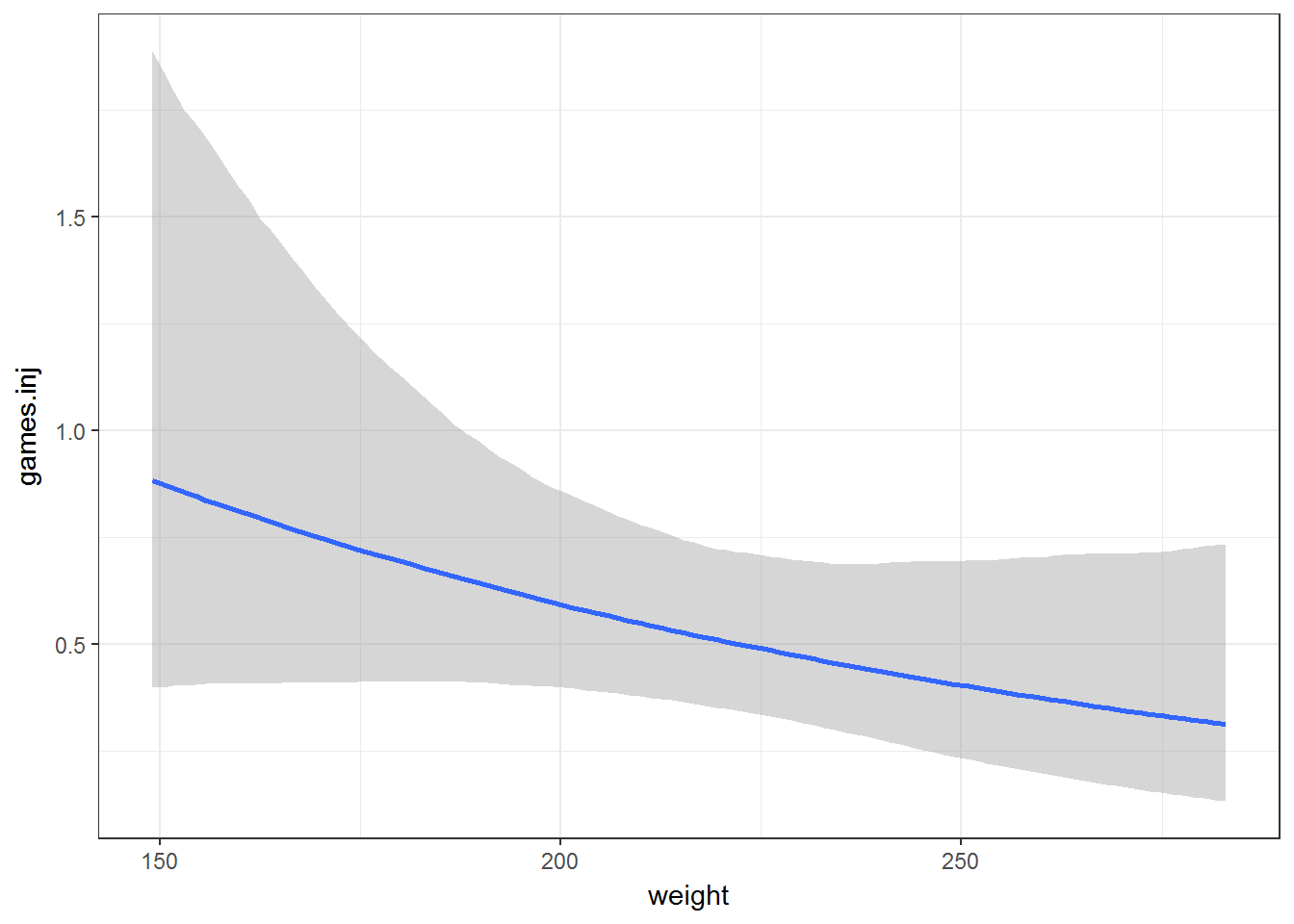
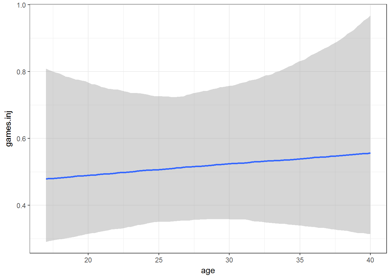
It’s really easy to get marginal effect plots in brms. The estimates show an incredibly strong yearly trend due to under reporting for 2015, 2016 in the data.
marginal_effects(fit0, ask = FALSE)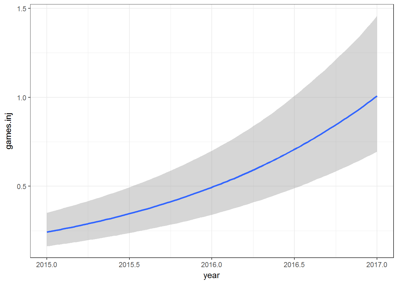

Simple Simulation
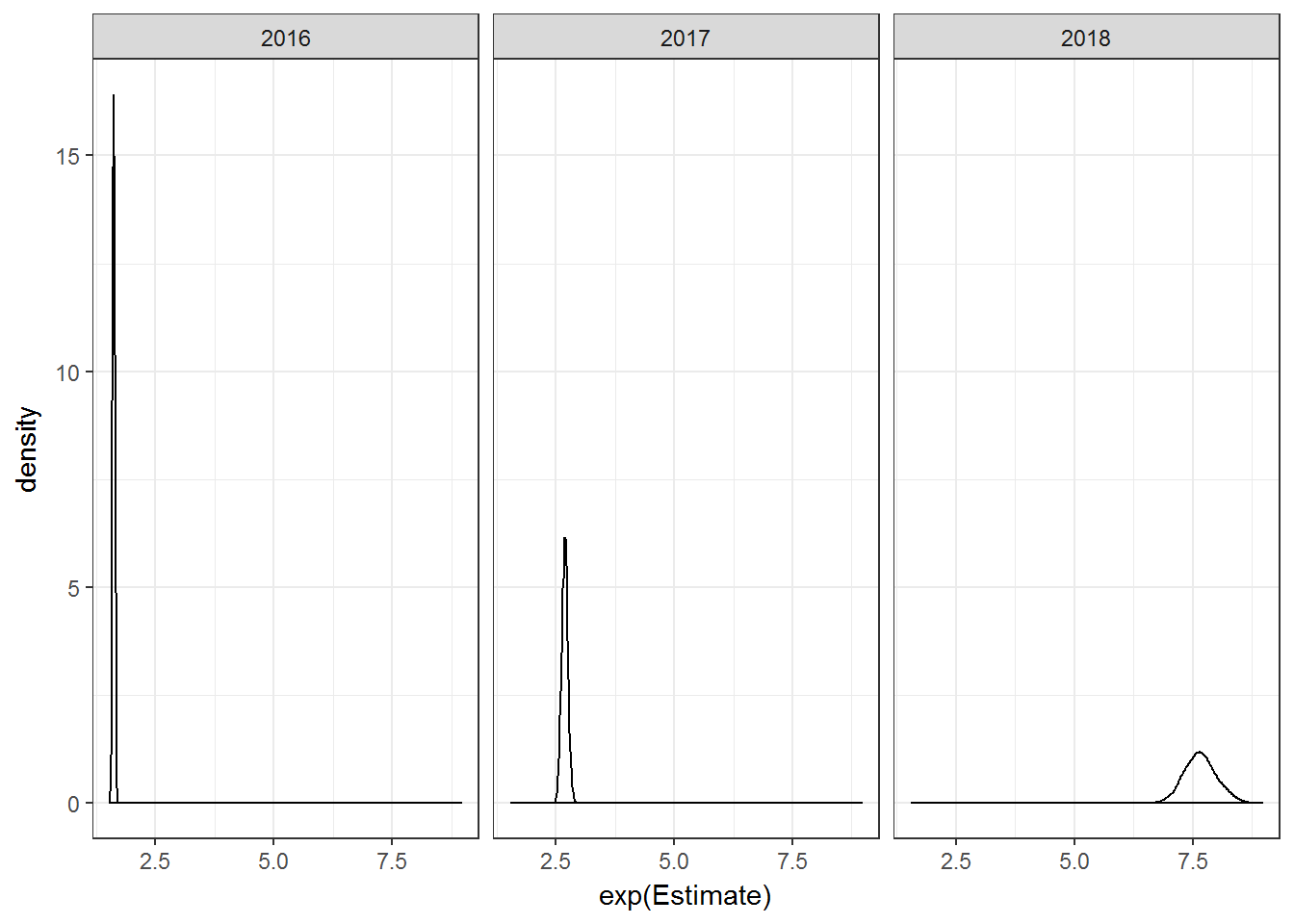
One interesting application of the model would be to simulate the expected number of games missed for a particular player. I try to do that for Antonio Brown below. I wanted to see how ridiculous the yearly extrapolation was so I predicted the expected number of missed games for Brown in 2016, 2017, and finally 2018. It’s clear that the model is primarily driven by the unrealistic yearly trend in the data.
sim.data <- data.frame(year = c(rep(2016, 1000),rep(2017,1000),rep(2018, 1000)),
                       pos1 = rep("WR", 3000),
                       height = rep(70, 3000),
                       weight = rep(186, 3000),
                       age = c(rep(28, 1000),rep(29,1000),rep(30,1000)),
                       player = rep("AB-3500", 3000))

abrown.pred <- predict(fit0, newdata = sim.data)

ggplot(data.frame(abrown.pred,year = c(rep(2016, 1000),rep(2017,1000),rep(2018, 1000))),
       aes(exp(Estimate))) + geom_density() + facet_wrap( ~ year)