Anyone trying to learn how to build and assess prediction models is immediately swamped with a litany of strange sounding performance metrics. In the binary outcome case you might encounter: sensitivity, specificity, precision, recall, accuracy, just to name a few. Fundamentally, all of the measures listed require the analyst to provide a category label for each element predicted. This is sometimes provided automatically with an algorithm. Or if the output of the model is a probability, a cut off is chosen and all elements below the cut off are classified one way, and all those above the other way. The probability cutoff that maximizes one or the other metric is then chosen. But how to choose which one or more of these metrics and why?
Instead of answering this question I’m going to argue that the question is misplaced. None of the metrics above is (solely or jointly) appropriate for model evaluation and that choosing a probability cutoff so as to optimize one or the other metric is often misguided. I’ll argue instead that the assessment of prediction methods should rely on (at least) two measures of quality, discrimination and calibration, and that these measures are jointly considered by using what are called proper scoring rules. Importantly, good performance on both metrics does not imply the model is useful. For the sake of simplicity, I’m only going to cover the binary outcome case though the conclusions can be extended to any outcome. In the event that a yes/no or class label decision is required, since probabilities can be difficult to work with and require judgement, the cutoff(s) should be chosen based on the relative costs and benefits of applying the separate labels. This is fundamentally a decision theory problem outside the scope of this post.
Discrimination and Calibration
In binary classification (prediction) problems, the primary focus for predictive performance is on discrimination. All of the measures previously listed, as well as other (better) measures like AUC (aka c-statistic), can be thought of as measures of discrimination. Discrimination measures compare the probability point estimates between classes. The more separation between the classes the better the discrimination.
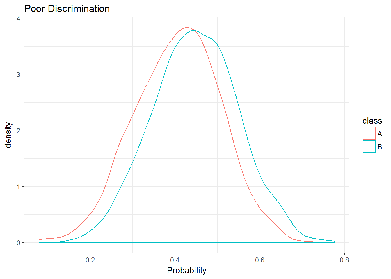
Imagine you have observed whether an event occurs in 2000 thousand patients. It just so happens that the event occured in 1000 patients and did not occur in the other 1000. You’re interested in predicting whether this event will occur in the future for unobserved patients, so you’ve built a prediction model. To get an idea of how well your method works you make predictions on new patients using your method and compare the predictions to their observed outcomes. In terms of discrimination, what you would like is for the method to assign a higher probability to patients who in fact did have an event. If you wanted to visually compare these predicted probabilities, you could use plots like those below. 

The first plot shows a cleaner separation between distributions of predictions and thus better discrimination. The second plot is labeled poor discrimination, but this is possibly a misnomer. Depending on the application, this might represent a valuable degree of separation. Probably the most common measure of discrimination is the area under the receiver operator curve (AUC), also referred to as the concordance probability (c-statistic or c-index). The “Good” plot above has an AUC of about .93, whereas the “Poor” plot has one of .64. If the two classes overlapped exactly, the AUC equals .5. In mathematical notation: \(AUC = Pr(\pi_i > \pi_j) + 1/2 * Pr(\pi_i = \pi_j)\), where i is an event occurs and j is no event occurs. Measures of discrimination like AUC are maximized when there is no overlap in the distribution of predicted values. Thus, the distance between predictions is not of interest but rather the ordering along the x-axis.
To take an extreme example, imagine that 1/2 of the new patients have an event and your method gives a probability of .01 to all the patients that didn’t experience an event and a probability of .02 to all the patients that did. This method has perfect discrimination but also the ludicrious interpretation that all patients have a risk of less than .02 even though 1/2 of all patients had an event. This suggests that what we’d like to have in addition to discrimination, is a measure of the accuracy of our probability predictions. This measure is referred to as calibration or reliability.
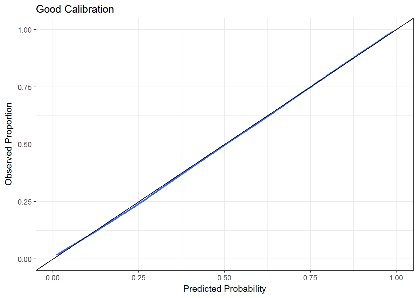
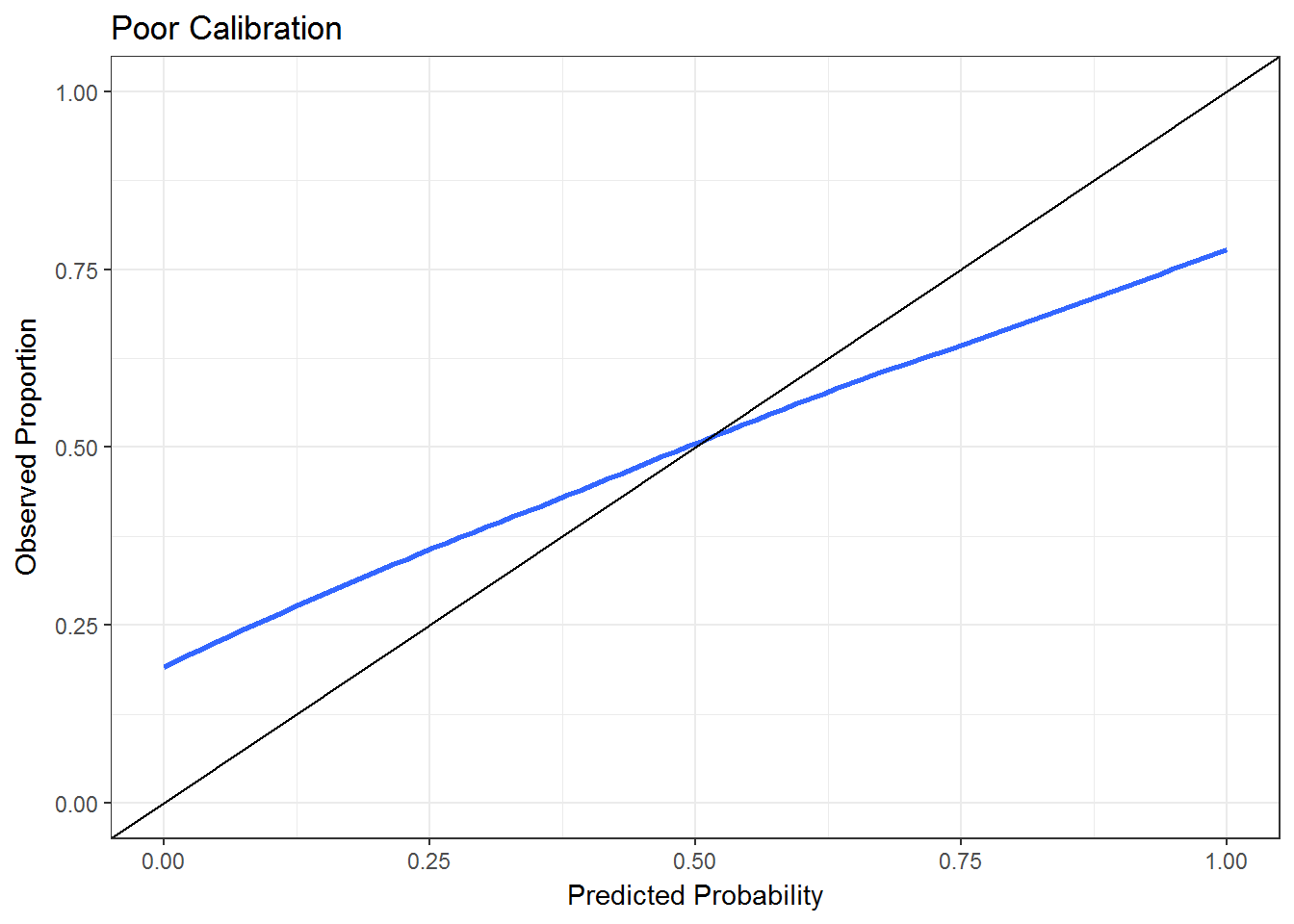
Good calibration means that on average \(\pi_i\) * 100 percent of events occur with predicted probability \(\pi_i\). To give an example, 50% of the patients with predicted probability of .5 or less should have events. Ideally, this should hold for the entire range [0,1]. Thus, calibration makes use of the entire range of predictions and the uncertainty involved in each class prediction. There are quantitative measures of calibration, but it is most easily inspected with a calibration or reliability plot. This can be done by using a loess smoother. Examples of good and poor calibration plots are shown below.


Scoring Rules
Scoring rules assign a number to the predicted probability and the actual outcome such that a scoring rule is proper if the expected (average) score is optimized by the true data generating process. It is strictly proper if it is uniquely optimized by the true data generating process. To put it more plainly, the true probability model will provide the best value of the proper scoring rule (though there may be ties with other models), whereas the strictly proper scoring rule will give the best value to the true probability model and no other. Proper scoring rules can be decomposed into separate components representing calibration and discrimination. Thus, by assessing models via proper scoring rules you can simultaneously consider model discrimination and calibration.
Two strictly proper scoring rules relevant to binary outcome prediction are the brier or quadratic scoring rule and logarithmic scoring rule. The brier score measures the squared difference between the observed outcome and predicted probability, \[(y_i - \pi_i)^2\] This measure is optimized at 0, representing perfect prediction. The logarithmic score is \[-ln(\pi_i) \] The logarithmic score is related to the likelihood function for binary outcome models and is closely related to the concept of entropy in information theory. The logarithmic rule gives more weight to extreme predictions (those near 0 and 1) than the brier score. Both measures provide valuable information about a models forecasting ability and in general should be preferred to other metrics that only measure discrimination (for instance AUC), or that require providing an outcome label instead of a probability (the litany of measures listed at the beginning of the post).
Additional Resources
Nice discussion of classification and scoring rules by Frank Harrell
The textbook Applied Statistical Inference by Leonhard Held has a nice and short chapter on prediction assessment.