Simple example of fitting splines with mixed models

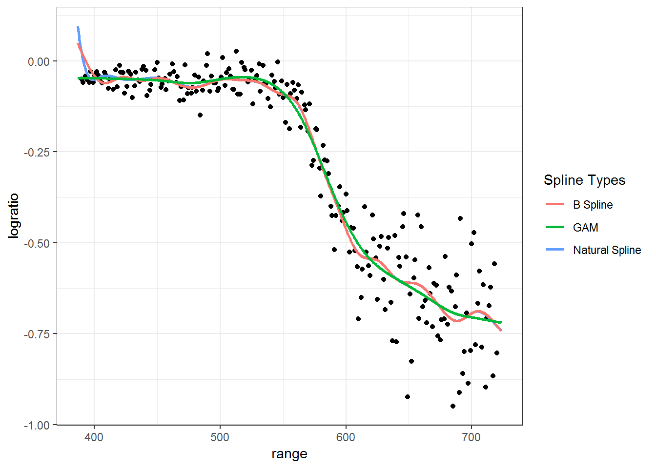
I thought it might be value to provide some code showing how splines can be fit using mixed models.

library(tidyverse)

## Warning: package 'tidyverse' was built under R version 3.4.4

## -- Attaching packages ------------------------------------------------------------------------------------------------ tidyverse 1.2.1 --

## v ggplot2 3.0.0     v purrr   0.2.5
## v tibble  1.4.2     v dplyr   0.7.6
## v tidyr   0.8.0     v stringr 1.3.1
## v readr   1.1.1     v forcats 0.2.0

## Warning: package 'ggplot2' was built under R version 3.4.4

## Warning: package 'readr' was built under R version 3.4.4

## Warning: package 'purrr' was built under R version 3.4.4

## Warning: package 'dplyr' was built under R version 3.4.4

## Warning: package 'stringr' was built under R version 3.4.4

## -- Conflicts --------------------------------------------------------------------------------------------------- tidyverse_conflicts() --
## x dplyr::filter() masks stats::filter()
## x dplyr::lag()    masks stats::lag()

library(nlme)

## 
## Attaching package: 'nlme'

## The following object is masked from 'package:dplyr':
## 
##     collapse

library(splines)
library(mgcv)

## This is mgcv 1.8-23. For overview type 'help("mgcv-package")'.

####Options----
theme_set(theme_bw())

## Parsed with column specification:
## cols(
##   range = col_integer(),
##   logratio = col_double()
## )

####Create Basis Functions----
#Number of knots
knot_num <- 20
#Location of knots
knot_loc <- quantile(unique(data$range),
                                         #select quantiles except 1st (0) and last (1)
                                         seq(0,1, length= (knot_num + 2))[-c(1,(knot_num + 2))])

#Boundaries
a <- 1.01*min(data$range) - 0.01*max(data$range) 
b <- 1.01*max(data$range) - 0.01*min(data$range)

#B spline
basis_func <- bs(data$range, Boundary.knots = c(a,b), knots = knot_loc, degree = 3)
#Natural spline
basis_func2 <- ns(data$range, Boundary.knots = c(a,b), knots = knot_loc, df = 4)

####Fit mixed Model----
intercept <- rep(1, length(data$range))

fit <- lme(logratio ~ range, data = data,
                     random = list(intercept = pdIdent(~-1+basis_func)))

fit2 <- lme(logratio ~ range, data = data,
                     random = list(intercept = pdIdent(~-1+basis_func2)))

#estimates
#B spline
beta_hat <- fit$coef$fixed

u_hat <- unlist(fit$coef$random)

sigma_square_e <- fit$sigma^2

sigma_square_u <- as.numeric(VarCorr(fit)[1,1])

#Natural Spline
beta_hat2 <- fit2$coef$fixed

u_hat2 <- unlist(fit2$coef$random)

sigma_square_e2 <- fit2$sigma^2

sigma_square_u2 <- as.numeric(VarCorr(fit2)[1,1])

#####Plot fit on a grid-----
# create the grid where you want to plot the function
grid_x <- seq(a,b, length = 1001)
#nx2 matrix of vector of 1s and values of grid
x_vals <- cbind(rep(1,1001),grid_x) 
#grid basis function
basis_func_grid <- bs(grid_x, Boundary.knots = c(a,b), knots = knot_loc, degree = 3)
basis_func_grid2 <- ns(grid_x, Boundary.knots = c(a,b), knots = knot_loc, df = 4)
# Get the function fit to the grid
grid_fit <- as.vector(x_vals%*%beta_hat + basis_func_grid%*%u_hat)
grid_fit2 <- as.vector(x_vals%*%beta_hat2 + basis_func_grid2%*%u_hat2)
#mgcv fit
gam_fit <- gam(logratio ~ s(range, bs = "cr", k = 20), method = "REML", data = data)
gam_grid <- predict(gam_fit, newdata = data.frame(range = grid_x))

#Plot smooth curves
spline_data <- data_frame(grid_x, grid_fit, grid_fit2, gam_grid)

data %>% ggplot(aes(x = range, y = logratio)) + geom_point() +
    geom_line(data = spline_data, aes(x = grid_x, y = grid_fit, color = "Natural Spline"), size = 1) +
    geom_line(data = spline_data, aes(x = grid_x, y = grid_fit2, color = "B Spline"), size = 1) +
  geom_line(data = spline_data, aes(x = grid_x, y = gam_grid, color = "GAM"), size = 1) +
  scale_color_discrete(name = "Spline Types")