Stan Basics

Simple one parameters models

I figured it would be valuable to start with coding some simple one parameter models where the answer can be known analytically (you can solve the answer by hand). Stan is typically used for some really cool stuff, but that can be intimidating if you’re just trying to dabble. The two simple examples I chose were from Jim Albert’s book Bayesian Computation with R. The first is a normal model with known mean and unknown variance and the second is a poisson model with an unknown rate parameter.

Normal model with known mean and unknown Variance

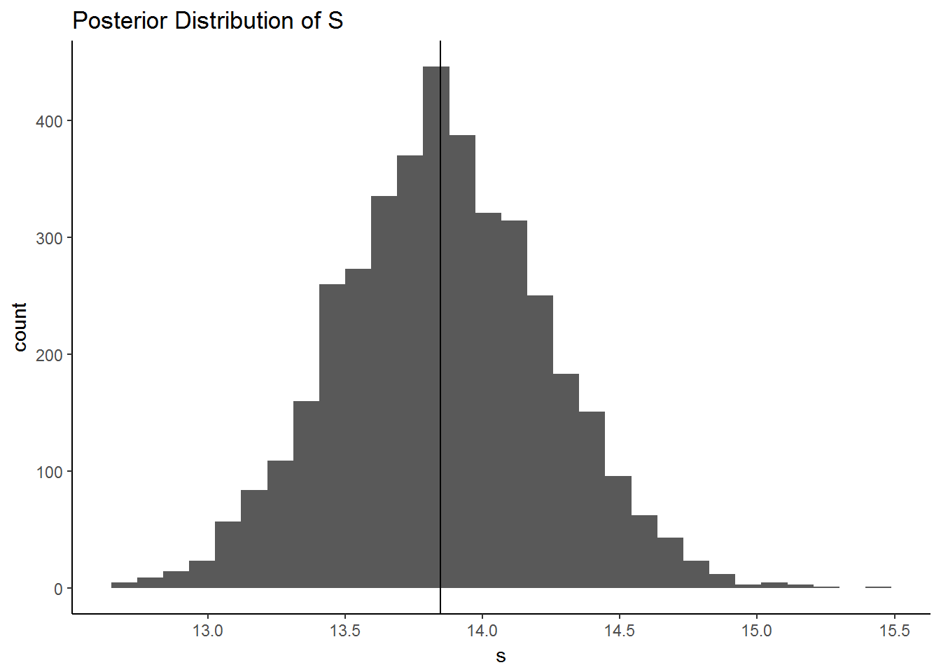
Albert provides the example of comparing the difference in American football game scores and published point spread. If we assume that the difference is from a normal distribution with mean 0 and unknown variance and we use an “uninformative” prior on \(\sigma^2\), \(p(\sigma^2) = 1/\sigma^2\), then \(p(\sigma^2 | data)\) has a known posterior (inverse chi-square) (See Albert’s book, pg. 40 Second edition for details). The code below is provided by Albert and samples from this posterior. I additionally plot a histogram of the posterior and print the .025, .5, and .975 quantiles of the distribution.

library(ggplot2)
library(LearnBayes)
data("footballscores")
d <- with(footballscores, favorite - underdog - spread)
n <- nrow(footballscores)
v <- sum(d^2)

#Standard deviation posterior
P <- rchisq(4000, n)/v
s <- sqrt(1/P)
qplot(s, geom = "histogram", 
      main = "Posterior Distribution of S") +
  geom_vline(xintercept = quantile(s, .5)) +
  theme_classic()

## `stat_bin()` using `bins = 30`. Pick better value with `binwidth`.

#Interval
quantile(s, c(.025,.5,.975))

##     2.5%      50%    97.5% 
## 13.11059 13.84735 14.62605

Now we can fit the same model in Stan. Using Stan in R requires installing the package RStan. You can pass Stan code to the stan function in Rstan as a string, or you can write your stan code separately and save it as .stan and use the file argument in the stan function. I think it’s easier to do the latter. You can write and edit Stan code in Rstudio by simply opening up a new text file. Once the file is saved as .stan, the syntax highlighting should start.

The stan function requires you to pass the data as a list and an argument for the location of your stan file.

library(rstan)

data.list <- list(n = n, d = d)

stan.samples <- stan(file = "code\\normal_unknown_variance.stan", 
                     data = data.list,
                     iter = 4000)

The stan code for the model is below. As can be seen, Stan requires a few blocks of code in addition to the code specifying the model. I left the prior for the variance as unspecified. Stan uses a default in that situation.

## 
## data {
##   int<lower = 0> n;
##   vector[n] d;
## }
## //Unknown parameters: Variance
## parameters {
##   real<lower = 0> S;
## }
## 
## model {
##   d ~ normal(0, sqrt(S));
## }
## 
## generated quantities {
##     real s;
##     s = sqrt(S);
## }

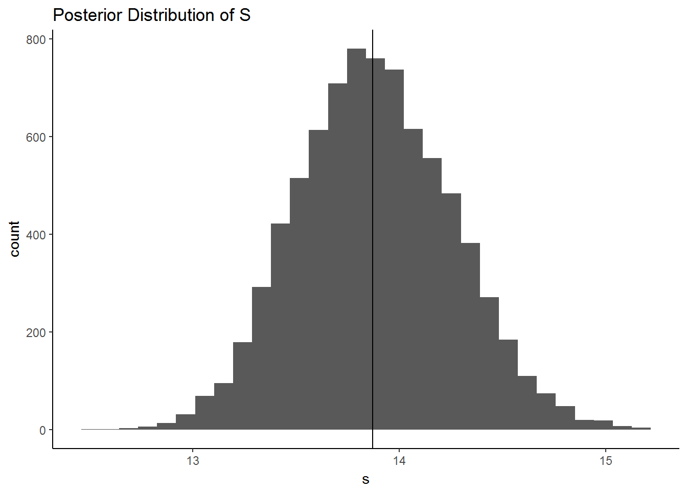
The stan.samples object contains draws from the posterior, which can be used to make inferences about our unknown parameter as well as check fit diagnostics. I plotted the draws as a histogram and printed the same quantiles as before.

#posterior inference
posterior <- as.data.frame(stan.samples)
with(posterior,
  qplot(s, geom = "histogram",
      main = "Posterior Distribution of S") + geom_vline(xintercept = quantile(s, .5)) +
      theme_classic()
)

## `stat_bin()` using `bins = 30`. Pick better value with `binwidth`.

quantile(posterior$s, c(.025, .5, .975))

##     2.5%      50%    97.5% 
## 13.18149 13.87012 14.63985

The histogram from the posterior derived from Stan is very similar to the analytically derived one above. The quantiles match very closely as well. The slight differences may have to do with the default prior for Stan being slightly different than that used by Albert, or could simply be sampling error since we only used a limited number of samples for both esimates.

Poisson model with unknown rate

The second example from Albert’s book involves estimating the mortality rate of heart transplants from a hospital. Since we’re dealing with counts, a natural starting point is with a poisson likelihood. The gamma distribution is a conjugate prior for the poisson likelihood. The prior Albert uses is \(gamma(alpha = 16, beta = 15174)\), and I’m going to use it as well. The set up for this problem involves two measurements, the number of heart transplant failures, yobs, and the total number of heart transplants, exposures. The code below draws samples from the posterior, \(p(\lambda | data)\), which is known to be \(gamma(alpha = 16 + yobs, beta = 15174 + exposures)\).

alpha <- 16
beta <- 15174
yobs <- 1
exposure <- 66

lambda <- rgamma(1000, shape = alpha + yobs, rate = beta + exposure)
qplot(lambda, geom = "histogram", 
      main = "Posterior Distribution of lambda") + 
        geom_vline(xintercept = quantile(lambda, .5)) +
  theme_classic()

## `stat_bin()` using `bins = 30`. Pick better value with `binwidth`.

quantile(lambda, c(.025,.5,.975))

##         2.5%          50%        97.5% 
## 0.0006496529 0.0010801951 0.0017239690

The stan code to fit the same model is below. In the data block I initialize 4 variables, the two parameters for the gamma prior, alpha and beta, and then the actual data, yobs and exposure. The values for these variables are provided as a list for the data argument of the stan function.

data.list <- list(alpha = alpha, beta = beta, yobs = yobs, ex = exposure)

stan.samples.poisson <- stan(file = "code\\poisson_rate.stan", 
                          data = data.list,
                          iter = 4000)

The resulting posterior distribution is plotted below and the 2.5, .5, and 97.5 quantiles are printed.

#posterior inference
posterior <- as.data.frame(stan.samples.poisson)
with(posterior,
  qplot(lambda, geom = "histogram",
      main = "Posterior Distribution of lambda") + 
      geom_vline(xintercept = quantile(lambda, .5)) +
      theme_classic()
)

## `stat_bin()` using `bins = 30`. Pick better value with `binwidth`.

quantile(posterior$lambda, c(.025, .5, .975))

##         2.5%          50%        97.5% 
## 0.0006560578 0.0011007345 0.0017319650

As before, the results are very similar, suggesting that I (hopefully!) set up the models in stan correctly. The actual stan code for the poisson model is printed below.

## //Define data going into model
## data {
##   int<lower = 0> yobs;
##   int<lower = 0> ex;
##   real<lower = 0> alpha;
##   real<lower = 0> beta;
## }
## //Unknown parameters: lambda
## parameters {
##   real<lower = 0> lambda;
## }
## //Model
## model {
##   lambda ~ gamma(alpha, beta);
##   yobs ~ poisson(ex*lambda);
## }

Conclusion

Hopefully, seeing the code for these simple models is helpful for anyone reading this. Writing Stan code for such simple models is obviously overkill (and tedious). But it was helpful since I already knew what the answers were supposed to be. I plan to move on to fitting more complicated regression models in Stan next.