Introduction
Super Learning is a conceptually simple way of combining predictions from different models using cross validation. It simply uses the cross-validated results to form an optimal weighted combination of predictions. Combining predictions across models, typically refered to as stacking or stacked ensembles, is not new. I’ve seen references as far back as about 30 years, though I wouldn’t be surprised if it was much older. However, as far as I know, it was only relatively recently (within 15 years) that some nice theoretical properties were proven for a particular type of stacking called super learning. The paper by Mark van der Laan establishing the results for the super learner can be found here Super Learner by Mark van der Laan.
I learned about super learning by attending a short course at Harvard school of public health led by Dr. Sherri Rose and Dr. Laura Hatfield. Dr. Rose gave a very nice presentation on the super learner and a few examples using it from her own research. The thing that really stood out to me about this method was its unification of the prediction model building process. There is no longer a need to pick a single model as best. This can be particularly difficult if several models perform similarly. The super learner will typically perform as good as the single best performing model and often better. Below I work through building a super learner from scratch.
A few resources I found very helpful for this are Stacked Generalizations by Ashley Naimi and Laura Balzer, the github for the paper, and the github for the SuperLearner package in R. Good chunks of the code below are taken and slightly edited from the Naimi and Balzer github. Additionally, datacamp published a nice article a few days ago walking through the SuperLearner package datacamp. datacamp is a great and cost effective way of learning about programming, statistics, and machine learning. I’ve used it in the past and recommend it, especially for beginners.
Super Learning from Scratch
The data
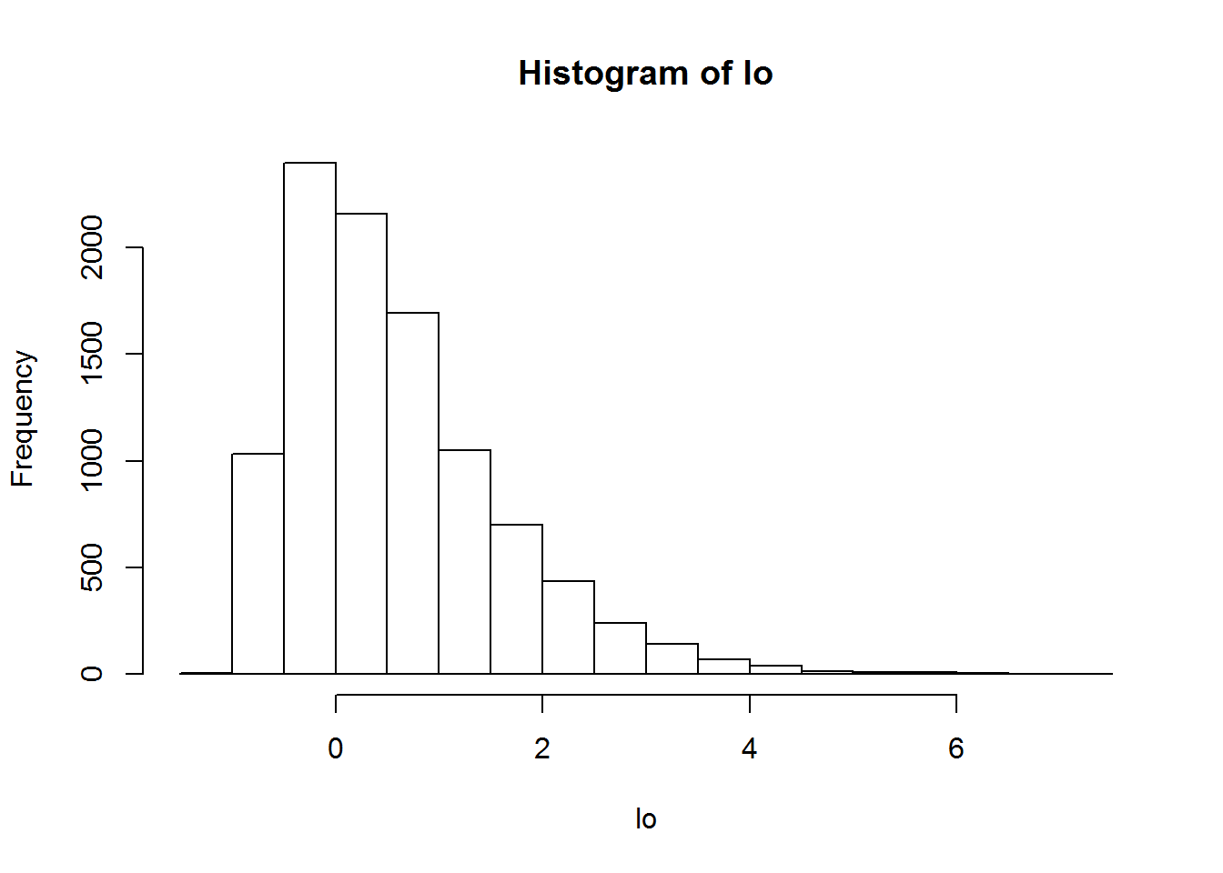
I generated 10,000 rows and 5 variables of fake data for this example using a multivariate normal. I then added a 6th variable by squaring the first variable and a 7th variable as the interaction between the 2nd and 3rd. I then randomly generated coefficients between -.5 and .5. The outcome will be binary, and thus a bernoulli random variable. The probability of an event will be the inverse logit of the linear combination of randomly generated coefficients and my fake data. Even though the logit scale (log odds) runs from negative infinity to infinity, essentially anything above or below 6 and negative 6 are very close to 1 and 0 on the probability scale. This will cause problems when I optimize the loss functions below, so I’ve tried to restrict the data generation to non-extreme values. You can see that in the histogram of log odds below.
library(rms)## Loading required package: Hmisc## Loading required package: lattice## Loading required package: survival## Loading required package: Formula## Loading required package: ggplot2##
## Attaching package: 'Hmisc'## The following objects are masked from 'package:base':
##
## format.pval, units## Loading required package: SparseM##
## Attaching package: 'SparseM'## The following object is masked from 'package:base':
##
## backsolvelibrary(mvtnorm)
library(Matrix)
library(SuperLearner)## Loading required package: nnls## Super Learner## Version: 2.0-22## Package created on 2017-07-18#Randomly generate data
set.seed(1256)
N = 10000
NVAR <- 5
#Covariance Matrix
sigma <- matrix(runif(NVAR^2,0,1), ncol=NVAR)
sigma <- forceSymmetric(sigma)
sigma <- as.matrix(nearPD(sigma)$mat)
#Mean vector:
mu <- round(runif(NVAR,-1,.1),2)
print(mu)## [1] -0.46 -0.47 -0.27 -0.94 -0.75#Generate data
X <- rmvnorm(N, mean=mu, sigma=sigma)
X <- cbind(X,X[,1]^2)
X <- cbind(X,X[,2]*X[,3])
coefs <- round(runif(NVAR+2, -.5, .5),2)
#Outcome
lo <- X %*% coefs
hist(lo)
#Extreme probabilities will make optimization more difficult
pr <- exp(lo)/(1 + exp(lo))

Y <- rbinom(N, size = 1,pr = pr)
Exploring the data
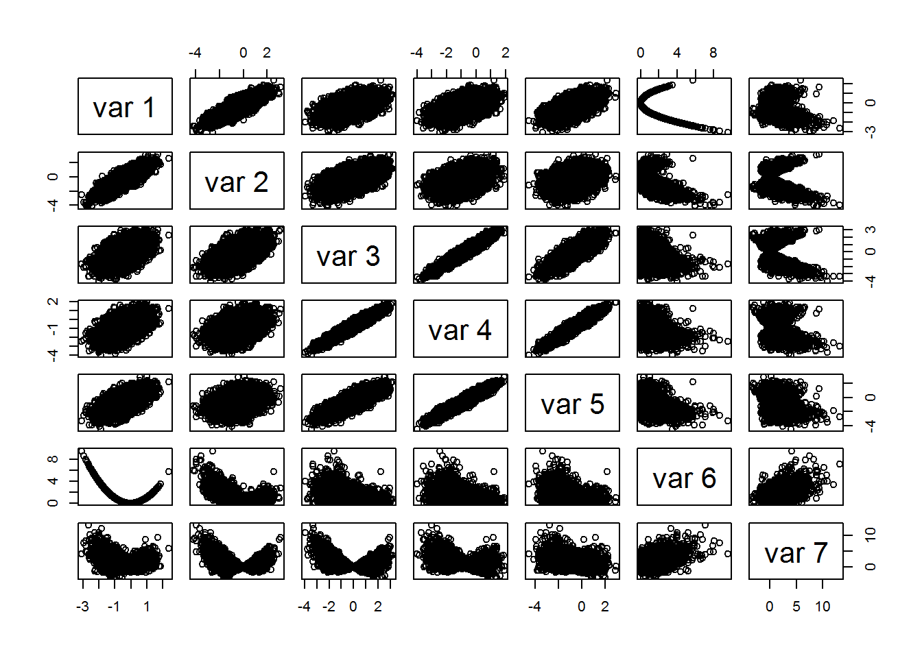
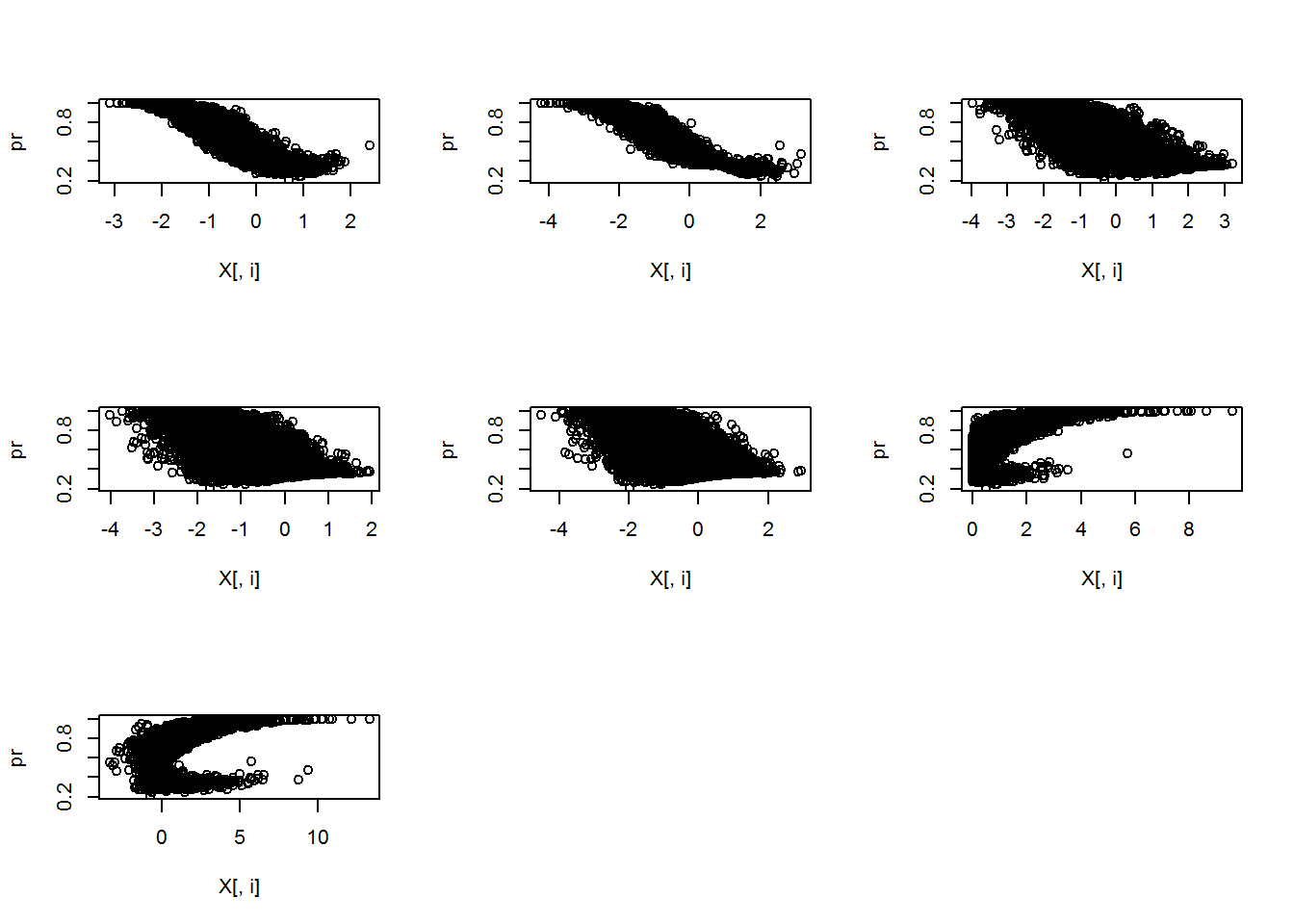
I generated a summary table of the 7 predictor variables as well as a pairs plot. Additionally, I plotted the probability of an event as a function of each predictor variable. The plots show some nice looking relationships, but this is fake data so we won’t dwell on it much. However, it’s always good to exploratory analysis before fitting your models.
#Exploratory plots
summary(X)
## V1 V2 V3 V4
## Min. :-3.094573 Min. :-4.2007 Min. :-3.9632 Min. :-4.0099
## 1st Qu.:-0.903185 1st Qu.:-1.1385 1st Qu.:-0.9596 1st Qu.:-1.4806
## Median :-0.460482 Median :-0.4630 Median :-0.2677 Median :-0.9303
## Mean :-0.457468 Mean :-0.4705 Mean :-0.2581 Mean :-0.9285
## 3rd Qu.:-0.004579 3rd Qu.: 0.1893 3rd Qu.: 0.4380 3rd Qu.:-0.3772
## Max. : 2.393029 Max. : 3.1435 Max. : 3.2037 Max. : 1.9370
## V5 V6 V7
## Min. :-4.5139 Min. :0.00000 Min. :-3.31823
## 1st Qu.:-1.3520 1st Qu.:0.07253 1st Qu.:-0.03143
## Median :-0.7373 Median :0.32206 Median : 0.24488
## Mean :-0.7367 Mean :0.66349 Mean : 0.68102
## 3rd Qu.:-0.1089 3rd Qu.:0.90247 3rd Qu.: 1.03135
## Max. : 2.9404 Max. :9.57638 Max. :13.27604pairs(X)
par(mfrow = c(3,3))
invisible(lapply(1:ncol(X), function(i) plot(X[,i],pr)))
Fitting the super learner using the SuperLearner package
The super learner function syntax is fairly straight forward and similar to fitting any other model. The biggest difference is the SL.library, the list of candidate algorithms for the super learner to build. The package comes with build in wrapper functions (all the models with SL. in from of the name) for a fairly wide variety of models. If you want to use other models, or specify particular tuning parameters, you’ll need to write your own wrapper functions. The datacamp tutorial helpfully covers that.
The candidate models I’m going to use are a main effects glm, linear discriminate analysis (lda), quadratic discriminate analysis (qda), and a random forest (using the ranger package). I fit the super learner twice, each with a separate loss function. The first is rank loss (AUC), while the second is the negative log likelihood. I’m just going to store the results and compare them to what I derive manually. The results we get should be very similar to what the function produces.
#Super Learner

DAT <- data.frame(X[,1:5])

SL.library <- c("SL.glm",
                "SL.lda",
                "SL.qda",
                "SL.ranger")


system.time({
  sl.AUC = SuperLearner(Y = Y, X = DAT,
                    family = binomial(),
                    method = "method.AUC",
                    SL.library = SL.library)
})
## Loading required package: cvAUC## Loading required package: ROCR## Loading required package: gplots##
## Attaching package: 'gplots'## The following object is masked from 'package:stats':
##
## lowess## Loading required package: data.table## ## cvAUC version: 1.1.0## Notice to cvAUC users: Major speed improvements in version 1.1.0## ## Loading required package: MASS## Loading required package: ranger## user system elapsed
## 136.70 1.97 135.03system.time({
sl.LL = SuperLearner(Y = Y, X = DAT,
family = binomial(),
method = "method.NNloglik",
SL.library = SL.library)
})## user system elapsed
## 132.44 1.45 130.37Manually building the super learner
The super learner is a weighted combination of the cross validated predictions of the candidate models. In the code below I perform 20 fold cross validation for the glm, lda, qda, and random forest models and store the results. I then combine these with the observed outcomes (vector of 1s and 0s) into a 10,000 by 5 matrix. In order to derive the super learner weights, you simply need to optimize your selected loss function. That is, use the optim function in R to find the coefficients that minimize or maximize the loss/objective function. I compute the weights for two loss functions: the rank loss (AUC) and negative log likelihood. I prefer the latter because it’s a proper scoring rule (won’t tell you a worse model is better). The weights are standardized so that they sum to one.
DATA <- data.frame(Y = Y, DAT)


#Create folds
folds <- 20
splt <- split(DATA,1:folds)


#Fit models
glm.mods <- lapply(1:folds, function(ii) glm(formula = Y ~ ., data = do.call(rbind, splt[-ii]), family="binomial"))
lda.mods <- lapply(1:folds, function(ii) lda(formula = Y ~ ., data = do.call(rbind, splt[-ii])))
qda.mods <- lapply(1:folds, function(ii) qda(formula = Y ~ ., data = do.call(rbind, splt[-ii])))
rf.mods <- lapply(1:folds, function(ii) ranger(formula = Y ~ ., data = do.call(rbind, splt[-ii])))

#Compute model Predictions

p.glm <- lapply(1:folds,function(ii) predict(glm.mods[[ii]], newdata = rbindlist(splt[ii]), type = "response"))
p.lda <- lapply(1:folds,function(ii) predict(lda.mods[[ii]], newdata = rbindlist(splt[ii]), type = "response"))
p.qda <- lapply(1:folds,function(ii) predict(qda.mods[[ii]], newdata = rbindlist(splt[ii]), type = "response"))
p.rf <- lapply(1:folds,function(ii) predict(rf.mods[[ii]], data = rbindlist(splt[ii]), type = "response"))


#Combine outcomes with prediction probabilities
Y.preds <- NULL
for(i in 1:folds){
  Y.preds[[i]]<-cbind(splt[[i]][,1],p.glm[[i]],p.lda[[i]]$posterior[,2],p.qda[[i]]$posterior[,2], p.rf[[i]]$predictions)
}


#Manually compute SL coefficients

cv.X <- data.frame(do.call(rbind,Y.preds),row.names=NULL); names(X)<-c("Y","GLM","LDA","QDA","RF")

bounds = c(0, Inf)

AUCF<-function(A, y, par){
  AUCC <- function(A,y,par) {
  A<-as.matrix(A)
  names(par)<-c("GLM","LDA","QDA","RF")
  predictions <- crossprod(t(A),par)
  1 - AUC(predictions = predictions, labels = y)
  }
  bounds = c(0, Inf)
  fit <- optim(par= par, fn=AUCC, A=A, y=y,
               method="L-BFGS-B",lower=bounds[1],upper=bounds[2])
  fit$par/sum(fit$par)

}

##Binomial negative log likelihood
NNloglik <- function(A, y, par) {
  A <- as.matrix(trimLogit(A, trim = 0.001))
  names(par) <- c("GLM","LDA","QDA","RF")
  fmin <- function(par, A, y) {
    p <- plogis(crossprod(t(A), par))
   -sum(2 * ifelse(y, log(p), log(1-p)))
  }
  gmin <- function(par, A, y) {
    names(par) <- c("GLM","LDA","QDA","RF")
    eta <- A %*% par
    p <- plogis(eta)
    -2 * t(dlogis(eta) * ifelse(y, 1/p, -1/(1-p))) %*% A
  }
  fit2 <- optim(par, fn = fmin, gr = gmin, A = A, y = y, method = "L-BFGS-B", lower = 0)
  fit2$par[fit2$par < 0] <- 0
  fit2$par[is.na(fit2$par)] <- 0
  print(fit2)
  print(fit2$par/sum(abs(fit2$par)))
}
Comparing manual weights with SuperLearner function weights
We can see that there are slight differences between the manual super learner weights and the weights from the function, but that they are overall fairly close.
#AUC Results
sl.AUC
##
## Call:
## SuperLearner(Y = Y, X = DAT, family = binomial(), SL.library = SL.library,
## method = "method.AUC")
##
##
## Risk Coef
## SL.glm_All 0.2750461 0.3337970
## SL.lda_All 0.2750400 0.3357307
## SL.qda_All 0.2753354 0.3304723
## SL.ranger_All 0.3241119 0.0000000AUCF(cv.X[,2:5], cv.X[,1], par = c(1/4,1/4,1/4,1/4))## [1] 0.3361015 0.3304125 0.3334860 0.0000000##Log likelihood Results
sl.LL ##
## Call:
## SuperLearner(Y = Y, X = DAT, family = binomial(), SL.library = SL.library,
## method = "method.NNloglik")
##
##
## Risk Coef
## SL.glm_All 0.5931421 0
## SL.lda_All 0.5931418 0
## SL.qda_All 0.5889857 1
## SL.ranger_All Inf 0NNloglik(par = c(1/4,1/4,1/4,1/4), A = cv.X[,2:5], y = cv.X[,1])## $par
## GLM LDA QDA RF
## 0.000000 0.000000 1.004494 0.000000
##
## $value
## [1] 11776.67
##
## $counts
## function gradient
## 12 12
##
## $convergence
## [1] 0
##
## $message
## [1] "CONVERGENCE: REL_REDUCTION_OF_F <= FACTR*EPSMCH"
##
## GLM LDA QDA RF
## 0 0 1 0